Free Statistics
of Irreproducible Research!
Description of Statistical Computation | |||||||||||||||||||||||||||||||||||||||||||||||||||||||||||||
|---|---|---|---|---|---|---|---|---|---|---|---|---|---|---|---|---|---|---|---|---|---|---|---|---|---|---|---|---|---|---|---|---|---|---|---|---|---|---|---|---|---|---|---|---|---|---|---|---|---|---|---|---|---|---|---|---|---|---|---|---|---|
| Author's title | |||||||||||||||||||||||||||||||||||||||||||||||||||||||||||||
| Author | *The author of this computation has been verified* | ||||||||||||||||||||||||||||||||||||||||||||||||||||||||||||
| R Software Module | rwasp_linear_regression.wasp | ||||||||||||||||||||||||||||||||||||||||||||||||||||||||||||
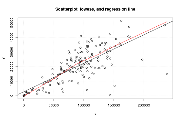
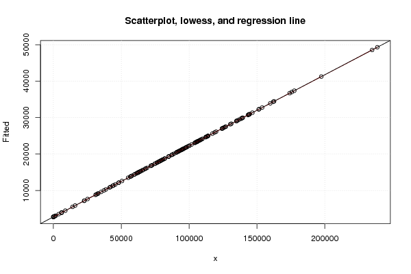
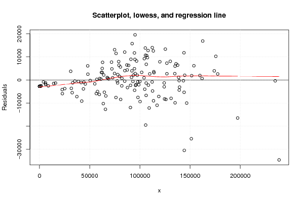
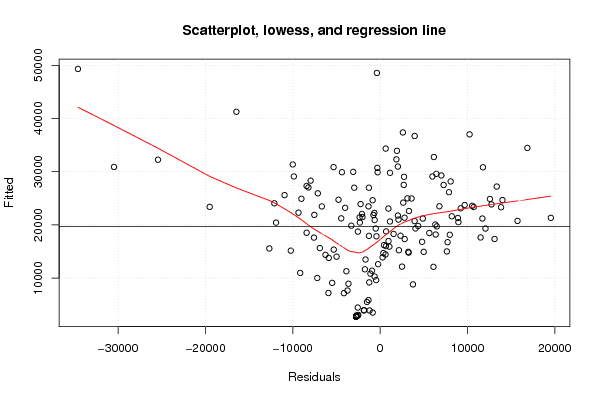
| Title produced by software | Linear Regression Graphical Model Validation | ||||||||||||||||||||||||||||||||||||||||||||||||||||||||||||
| Date of computation | Wed, 07 Dec 2011 14:04:17 -0500 | ||||||||||||||||||||||||||||||||||||||||||||||||||||||||||||
| Cite this page as follows | Statistical Computations at FreeStatistics.org, Office for Research Development and Education, URL https://freestatistics.org/blog/index.php?v=date/2011/Dec/07/t1323284706n2hhbjsdka1hjal.htm/, Retrieved Wed, 09 Jul 2025 12:40:01 +0000 | ||||||||||||||||||||||||||||||||||||||||||||||||||||||||||||
| Statistical Computations at FreeStatistics.org, Office for Research Development and Education, URL https://freestatistics.org/blog/index.php?pk=152619, Retrieved Wed, 09 Jul 2025 12:40:01 +0000 | |||||||||||||||||||||||||||||||||||||||||||||||||||||||||||||
| QR Codes: | |||||||||||||||||||||||||||||||||||||||||||||||||||||||||||||
|
| |||||||||||||||||||||||||||||||||||||||||||||||||||||||||||||
| Original text written by user: | |||||||||||||||||||||||||||||||||||||||||||||||||||||||||||||
| IsPrivate? | No (this computation is public) | ||||||||||||||||||||||||||||||||||||||||||||||||||||||||||||
| User-defined keywords | |||||||||||||||||||||||||||||||||||||||||||||||||||||||||||||
| Estimated Impact | 187 | ||||||||||||||||||||||||||||||||||||||||||||||||||||||||||||
Tree of Dependent Computations | |||||||||||||||||||||||||||||||||||||||||||||||||||||||||||||
| Family? (F = Feedback message, R = changed R code, M = changed R Module, P = changed Parameters, D = changed Data) | |||||||||||||||||||||||||||||||||||||||||||||||||||||||||||||
| - [Linear Regression Graphical Model Validation] [Colombia Coffee -...] [2008-02-26 10:22:06] [74be16979710d4c4e7c6647856088456] - RMPD [Linear Regression Graphical Model Validation] [] [2011-11-14 19:43:01] [d623f9be707a26b8ffaece1fc4d5a7ee] - PD [Linear Regression Graphical Model Validation] [] [2011-12-07 19:04:17] [47d38a19087200036e90a9f702d012f8] [Current] - [Linear Regression Graphical Model Validation] [] [2011-12-20 21:05:46] [74be16979710d4c4e7c6647856088456] - [Linear Regression Graphical Model Validation] [] [2011-12-20 21:05:46] [74be16979710d4c4e7c6647856088456] | |||||||||||||||||||||||||||||||||||||||||||||||||||||||||||||
| Feedback Forum | |||||||||||||||||||||||||||||||||||||||||||||||||||||||||||||
Post a new message | |||||||||||||||||||||||||||||||||||||||||||||||||||||||||||||
Dataset | |||||||||||||||||||||||||||||||||||||||||||||||||||||||||||||
| Dataseries X: | |||||||||||||||||||||||||||||||||||||||||||||||||||||||||||||
124252 98956 98073 106816 41449 76173 177551 22807 126938 61680 72117 79738 57793 91677 64631 106385 161961 112669 114029 124550 105416 72875 81964 104880 76302 96740 93071 78912 35224 90694 125369 80849 104434 65702 108179 63583 95066 62486 31081 94584 87408 68966 88766 57139 90586 109249 33032 96056 146648 80613 87026 5950 131106 32551 31701 91072 159803 143950 112368 82124 144068 162627 55062 95329 105612 62853 125976 79146 108461 99971 77826 22618 84892 92059 77993 104155 109840 238712 67486 68007 48194 134796 38692 93587 56622 15986 113402 97967 74844 136051 50548 112215 59591 59938 137639 143372 138599 174110 135062 175681 130307 139141 44244 43750 48029 95216 92288 94588 197426 151244 139206 106271 1168 71764 25162 45635 101817 855 100174 14116 85008 124254 105793 117129 8773 94747 107549 97392 126893 118850 234853 74783 66089 95684 139537 144253 153824 63995 84891 61263 106221 113587 113864 37238 119906 135096 151611 144645 0 6023 0 0 0 0 77457 62464 0 0 1644 6179 3926 42087 0 87656 | |||||||||||||||||||||||||||||||||||||||||||||||||||||||||||||
| Dataseries Y: | |||||||||||||||||||||||||||||||||||||||||||||||||||||||||||||
25695 19967 14338 34117 9713 10024 39981 1271 30207 18035 21609 19836 9028 21750 10038 30276 34972 19954 28113 18830 37144 17916 16186 19195 29124 29813 20270 26105 9155 18113 40546 10096 32338 2871 36592 4914 30190 18153 12558 32894 24138 16628 26369 14171 8500 11940 7935 19456 21347 24095 26204 2694 20366 3597 5296 29463 35838 42590 38665 19442 25515 51318 11807 24130 34053 22641 18898 24539 21664 21577 16643 3007 18798 24648 20286 23999 26813 14718 16963 16673 14646 31772 9648 23096 7905 4527 37432 21082 30437 36288 12369 23774 8108 15049 36021 30391 30910 40656 35070 47250 36236 29601 10443 7409 18213 40856 36471 26077 24797 6816 25527 22139 238 24459 3913 9895 25902 338 12937 3988 23370 24015 3870 14648 1888 16768 33400 23770 34762 18793 48186 20140 8728 19060 26880 415 38902 17375 31360 15051 16785 15886 28548 2805 34012 19215 34177 32990 0 2065 0 0 0 0 17428 19912 0 0 556 2089 2658 1801 0 16541 | |||||||||||||||||||||||||||||||||||||||||||||||||||||||||||||
Tables (Output of Computation) | |||||||||||||||||||||||||||||||||||||||||||||||||||||||||||||
| |||||||||||||||||||||||||||||||||||||||||||||||||||||||||||||
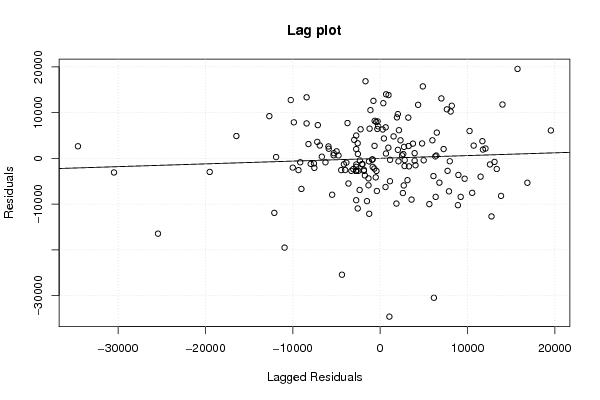
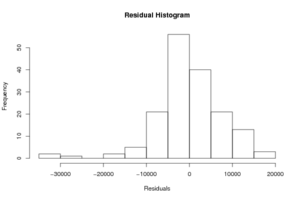
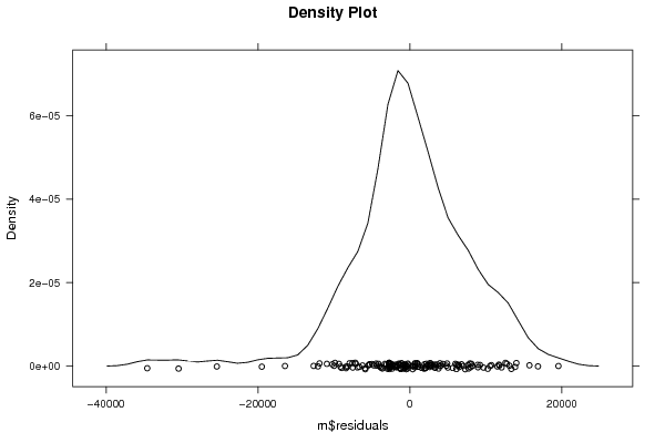
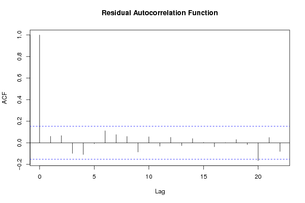
Figures (Output of Computation) | |||||||||||||||||||||||||||||||||||||||||||||||||||||||||||||
Input Parameters & R Code | |||||||||||||||||||||||||||||||||||||||||||||||||||||||||||||
| Parameters (Session): | |||||||||||||||||||||||||||||||||||||||||||||||||||||||||||||
| par1 = 0 ; | |||||||||||||||||||||||||||||||||||||||||||||||||||||||||||||
| Parameters (R input): | |||||||||||||||||||||||||||||||||||||||||||||||||||||||||||||
| par1 = 0 ; | |||||||||||||||||||||||||||||||||||||||||||||||||||||||||||||
| R code (references can be found in the software module): | |||||||||||||||||||||||||||||||||||||||||||||||||||||||||||||
par1 <- as.numeric(par1) | |||||||||||||||||||||||||||||||||||||||||||||||||||||||||||||