Repository of Reproducible Computations

Free Statistics

of Irreproducible Research!

Author's title

Author

*The author of this computation has been verified*

R Software Module

rwasp_arimaforecasting.wasp

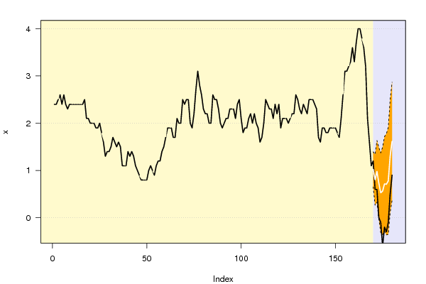
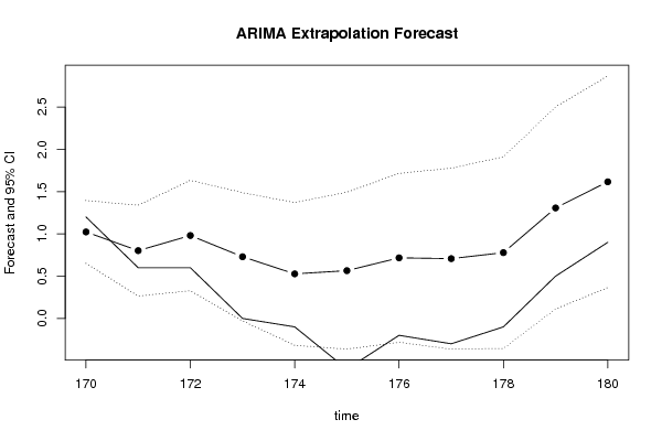
Title produced by software

ARIMA Forecasting

Date of computation

Tue, 06 Dec 2011 18:26:48 -0500

Cite this page as follows

Statistical Computations at FreeStatistics.org, Office for Research Development and Education, URL https://freestatistics.org/blog/index.php?v=date/2011/Dec/06/t132321405264p4vekjbvrp4bh.htm/, Retrieved Mon, 29 Apr 2024 03:59:47 +0000

Statistical Computations at FreeStatistics.org, Office for Research Development and Education, URL https://freestatistics.org/blog/index.php?pk=152038, Retrieved Mon, 29 Apr 2024 03:59:47 +0000

QR Codes:

Paste this QR Code to cite your computation.

Original text written by user:

IsPrivate?

No (this computation is public)

User-defined keywords

Estimated Impact

109

Family? (F = Feedback message, R = changed R code, M = changed R Module, P = changed Parameters, D = changed Data)

-     [Univariate Data Series] [data set] [2008-12-01 19:54:57] [b98453cac15ba1066b407e146608df68]
- RMP   [Standard Deviation-Mean Plot] [Unemployment] [2010-11-29 10:34:47] [b98453cac15ba1066b407e146608df68]
- RMP     [ARIMA Forecasting] [Unemployment] [2010-11-29 20:46:45] [b98453cac15ba1066b407e146608df68]
-   PD      [ARIMA Forecasting] [WS9 - ARIMA Forec...] [2010-12-04 16:25:58] [8ef49741e164ec6343c90c7935194465]
-   P         [ARIMA Forecasting] [WS9 - ARIMA Forec...] [2010-12-04 16:58:46] [8ef49741e164ec6343c90c7935194465]
- R PD          [ARIMA Forecasting] [WS9 - ARIMA Forec...] [2010-12-07 11:26:44] [1f5baf2b24e732d76900bb8178fc04e7]
-                 [ARIMA Forecasting] [WS9 - ARIMA Forec...] [2010-12-07 11:48:16] [1f5baf2b24e732d76900bb8178fc04e7]
- R P                 [ARIMA Forecasting] [Arima Forecasting] [2011-12-06 23:26:48] [0f9b7c3b8d01420b2751adc6f98a35df] [Current]

Feedback Forum

Post a new message

Dataseries X:

Download CSV

Histogram

Boxplots

2.4
2.4
2.5
2.6
2.4
2.6
2.4
2.3
2.4
2.4
2.4
2.4
2.4
2.4
2.4
2.4
2.5
2.1
2.1
2
2
2
1.9
1.9
2
1.8
1.6
1.3
1.4
1.4
1.5
1.7
1.6
1.5
1.6
1.5
1.1
1.1
1.1
1.4
1.3
1.4
1.3
1.1
1
0.9
0.8
0.8
0.8
0.8
1
1.1
1
0.9
1.1
1.2
1.2
1.4
1.5
1.7
1.9
1.9
1.9
1.7
1.7
2.1
2
2
2.5
2.4
2.5
2.5
2
1.9
2.2
2.7
3.1
2.8
2.6
2.3
2.2
2.2
2
2
2.6
2.5
2.5
2.3
2
1.9
2
2.1
2.1
2.3
2.3
2.3
2.1
2.4
2.5
2.1
1.8
1.9
1.9
2.1
2.2
2
2.2
2
1.9
1.6
1.7
2
2.5
2.4
2.3
2.3
2.1
2.4
2.2
2.4
1.9
2.1
2.1
2.1
2
2.1
2.2
2.2
2.6
2.5
2.3
2.2
2.4
2.3
2.2
2.5
2.5
2.5
2.4
2.3
1.7
1.6
1.9
1.9
1.8
1.8
1.9
1.9
1.9
1.9
1.8
1.7
2.1
2.6
3.1
3.1
3.2
3.3
3.6
3.3
3.7
4
4
3.8
3.6
3.2
2.1
1.6
1.1
1.2
0.6
0.6
0
-0.1
-0.6
-0.2
-0.3
-0.1
0.5
0.9

Summary of computational transaction
Raw Input	view raw input (R code)
Raw Output	view raw output of R engine
Computing time	2 seconds
R Server	'Herman Ole Andreas Wold' @ wold.wessa.net

\begin{tabular}{lllllllll}
\hline
Summary of computational transaction \tabularnewline
Raw Input & view raw input (R code)  \tabularnewline
Raw Output & view raw output of R engine  \tabularnewline
Computing time & 2 seconds \tabularnewline
R Server & 'Herman Ole Andreas Wold' @ wold.wessa.net \tabularnewline
\hline
\end{tabular}
%Source: https://freestatistics.org/blog/index.php?pk=152038&T=0

[TABLE]
[ROW][C]Summary of computational transaction[/C][/ROW]
[ROW][C]Raw Input[/C][C]view raw input (R code) [/C][/ROW]
[ROW][C]Raw Output[/C][C]view raw output of R engine [/C][/ROW]
[ROW][C]Computing time[/C][C]2 seconds[/C][/ROW]
[ROW][C]R Server[/C][C]'Herman Ole Andreas Wold' @ wold.wessa.net[/C][/ROW]
[/TABLE]
Source: https://freestatistics.org/blog/index.php?pk=152038&T=0

Globally Unique Identifier (entire table): ba.freestatistics.org/blog/index.php?pk=152038&T=0

As an alternative you can also use a QR Code:

The GUIDs for individual cells are displayed in the table below:

Summary of computational transaction
Raw Input	view raw input (R code)
Raw Output	view raw output of R engine
Computing time	2 seconds
R Server	'Herman Ole Andreas Wold' @ wold.wessa.net

Univariate ARIMA Extrapolation Forecast
time	Y[t]	F[t]	95% LB	95% UB	p-value(H0: Y[t] = F[t])	P(F[t]>Y[t-1])	P(F[t]>Y[t-s])	P(F[t]>Y[169])
157	3.2	-	-	-	-	-	-	-
158	3.3	-	-	-	-	-	-	-
159	3.6	-	-	-	-	-	-	-
160	3.3	-	-	-	-	-	-	-
161	3.7	-	-	-	-	-	-	-
162	4	-	-	-	-	-	-	-
163	4	-	-	-	-	-	-	-
164	3.8	-	-	-	-	-	-	-
165	3.6	-	-	-	-	-	-	-
166	3.2	-	-	-	-	-	-	-
167	2.1	-	-	-	-	-	-	-
168	1.6	-	-	-	-	-	-	-
169	1.1	-	-	-	-	-	-	-
170	1.2	1.0231	0.6516	1.3947	0.1754	0.3425	0	0.3425
171	0.6	0.8019	0.265	1.3388	0.2305	0.0731	0	0.1382
172	0.6	0.9808	0.3279	1.6337	0.1265	0.8735	0	0.3602
173	0	0.7298	-0.0287	1.4882	0.0297	0.6313	0	0.1693
174	-0.1	0.5272	-0.3173	1.3717	0.0728	0.8894	0	0.0918
175	-0.6	0.5651	-0.3628	1.493	0.0069	0.92	0	0.1293
176	-0.2	0.7166	-0.2829	1.716	0.0361	0.9951	0	0.226
177	-0.3	0.7073	-0.363	1.7777	0.0325	0.9517	0	0.2361
178	-0.1	0.7782	-0.3546	1.9111	0.0643	0.9689	0	0.2889
179	0.5	1.3071	0.1117	2.5025	0.0929	0.9895	0.0968	0.6329
180	0.9	1.6162	0.3646	2.8678	0.131	0.9598	0.5101	0.7906

\begin{tabular}{lllllllll}
\hline
Univariate ARIMA Extrapolation Forecast \tabularnewline
time & Y[t] & F[t] & 95% LB & 95% UB & p-value(H0: Y[t] = F[t]) & P(F[t]>Y[t-1]) & P(F[t]>Y[t-s]) & P(F[t]>Y[169]) \tabularnewline
157 & 3.2 & - & - & - & - & - & - & - \tabularnewline
158 & 3.3 & - & - & - & - & - & - & - \tabularnewline
159 & 3.6 & - & - & - & - & - & - & - \tabularnewline
160 & 3.3 & - & - & - & - & - & - & - \tabularnewline
161 & 3.7 & - & - & - & - & - & - & - \tabularnewline
162 & 4 & - & - & - & - & - & - & - \tabularnewline
163 & 4 & - & - & - & - & - & - & - \tabularnewline
164 & 3.8 & - & - & - & - & - & - & - \tabularnewline
165 & 3.6 & - & - & - & - & - & - & - \tabularnewline
166 & 3.2 & - & - & - & - & - & - & - \tabularnewline
167 & 2.1 & - & - & - & - & - & - & - \tabularnewline
168 & 1.6 & - & - & - & - & - & - & - \tabularnewline
169 & 1.1 & - & - & - & - & - & - & - \tabularnewline
170 & 1.2 & 1.0231 & 0.6516 & 1.3947 & 0.1754 & 0.3425 & 0 & 0.3425 \tabularnewline
171 & 0.6 & 0.8019 & 0.265 & 1.3388 & 0.2305 & 0.0731 & 0 & 0.1382 \tabularnewline
172 & 0.6 & 0.9808 & 0.3279 & 1.6337 & 0.1265 & 0.8735 & 0 & 0.3602 \tabularnewline
173 & 0 & 0.7298 & -0.0287 & 1.4882 & 0.0297 & 0.6313 & 0 & 0.1693 \tabularnewline
174 & -0.1 & 0.5272 & -0.3173 & 1.3717 & 0.0728 & 0.8894 & 0 & 0.0918 \tabularnewline
175 & -0.6 & 0.5651 & -0.3628 & 1.493 & 0.0069 & 0.92 & 0 & 0.1293 \tabularnewline
176 & -0.2 & 0.7166 & -0.2829 & 1.716 & 0.0361 & 0.9951 & 0 & 0.226 \tabularnewline
177 & -0.3 & 0.7073 & -0.363 & 1.7777 & 0.0325 & 0.9517 & 0 & 0.2361 \tabularnewline
178 & -0.1 & 0.7782 & -0.3546 & 1.9111 & 0.0643 & 0.9689 & 0 & 0.2889 \tabularnewline
179 & 0.5 & 1.3071 & 0.1117 & 2.5025 & 0.0929 & 0.9895 & 0.0968 & 0.6329 \tabularnewline
180 & 0.9 & 1.6162 & 0.3646 & 2.8678 & 0.131 & 0.9598 & 0.5101 & 0.7906 \tabularnewline
\hline
\end{tabular}
%Source: https://freestatistics.org/blog/index.php?pk=152038&T=1

[TABLE]
[ROW][C]Univariate ARIMA Extrapolation Forecast[/C][/ROW]
[ROW][C]time[/C][C]Y[t][/C][C]F[t][/C][C]95% LB[/C][C]95% UB[/C][C]p-value(H0: Y[t] = F[t])[/C][C]P(F[t]>Y[t-1])[/C][C]P(F[t]>Y[t-s])[/C][C]P(F[t]>Y[169])[/C][/ROW]
[ROW][C]157[/C][C]3.2[/C][C]-[/C][C]-[/C][C]-[/C][C]-[/C][C]-[/C][C]-[/C][C]-[/C][/ROW]
[ROW][C]158[/C][C]3.3[/C][C]-[/C][C]-[/C][C]-[/C][C]-[/C][C]-[/C][C]-[/C][C]-[/C][/ROW]
[ROW][C]159[/C][C]3.6[/C][C]-[/C][C]-[/C][C]-[/C][C]-[/C][C]-[/C][C]-[/C][C]-[/C][/ROW]
[ROW][C]160[/C][C]3.3[/C][C]-[/C][C]-[/C][C]-[/C][C]-[/C][C]-[/C][C]-[/C][C]-[/C][/ROW]
[ROW][C]161[/C][C]3.7[/C][C]-[/C][C]-[/C][C]-[/C][C]-[/C][C]-[/C][C]-[/C][C]-[/C][/ROW]
[ROW][C]162[/C][C]4[/C][C]-[/C][C]-[/C][C]-[/C][C]-[/C][C]-[/C][C]-[/C][C]-[/C][/ROW]
[ROW][C]163[/C][C]4[/C][C]-[/C][C]-[/C][C]-[/C][C]-[/C][C]-[/C][C]-[/C][C]-[/C][/ROW]
[ROW][C]164[/C][C]3.8[/C][C]-[/C][C]-[/C][C]-[/C][C]-[/C][C]-[/C][C]-[/C][C]-[/C][/ROW]
[ROW][C]165[/C][C]3.6[/C][C]-[/C][C]-[/C][C]-[/C][C]-[/C][C]-[/C][C]-[/C][C]-[/C][/ROW]
[ROW][C]166[/C][C]3.2[/C][C]-[/C][C]-[/C][C]-[/C][C]-[/C][C]-[/C][C]-[/C][C]-[/C][/ROW]
[ROW][C]167[/C][C]2.1[/C][C]-[/C][C]-[/C][C]-[/C][C]-[/C][C]-[/C][C]-[/C][C]-[/C][/ROW]
[ROW][C]168[/C][C]1.6[/C][C]-[/C][C]-[/C][C]-[/C][C]-[/C][C]-[/C][C]-[/C][C]-[/C][/ROW]
[ROW][C]169[/C][C]1.1[/C][C]-[/C][C]-[/C][C]-[/C][C]-[/C][C]-[/C][C]-[/C][C]-[/C][/ROW]
[ROW][C]170[/C][C]1.2[/C][C]1.0231[/C][C]0.6516[/C][C]1.3947[/C][C]0.1754[/C][C]0.3425[/C][C]0[/C][C]0.3425[/C][/ROW]
[ROW][C]171[/C][C]0.6[/C][C]0.8019[/C][C]0.265[/C][C]1.3388[/C][C]0.2305[/C][C]0.0731[/C][C]0[/C][C]0.1382[/C][/ROW]
[ROW][C]172[/C][C]0.6[/C][C]0.9808[/C][C]0.3279[/C][C]1.6337[/C][C]0.1265[/C][C]0.8735[/C][C]0[/C][C]0.3602[/C][/ROW]
[ROW][C]173[/C][C]0[/C][C]0.7298[/C][C]-0.0287[/C][C]1.4882[/C][C]0.0297[/C][C]0.6313[/C][C]0[/C][C]0.1693[/C][/ROW]
[ROW][C]174[/C][C]-0.1[/C][C]0.5272[/C][C]-0.3173[/C][C]1.3717[/C][C]0.0728[/C][C]0.8894[/C][C]0[/C][C]0.0918[/C][/ROW]
[ROW][C]175[/C][C]-0.6[/C][C]0.5651[/C][C]-0.3628[/C][C]1.493[/C][C]0.0069[/C][C]0.92[/C][C]0[/C][C]0.1293[/C][/ROW]
[ROW][C]176[/C][C]-0.2[/C][C]0.7166[/C][C]-0.2829[/C][C]1.716[/C][C]0.0361[/C][C]0.9951[/C][C]0[/C][C]0.226[/C][/ROW]
[ROW][C]177[/C][C]-0.3[/C][C]0.7073[/C][C]-0.363[/C][C]1.7777[/C][C]0.0325[/C][C]0.9517[/C][C]0[/C][C]0.2361[/C][/ROW]
[ROW][C]178[/C][C]-0.1[/C][C]0.7782[/C][C]-0.3546[/C][C]1.9111[/C][C]0.0643[/C][C]0.9689[/C][C]0[/C][C]0.2889[/C][/ROW]
[ROW][C]179[/C][C]0.5[/C][C]1.3071[/C][C]0.1117[/C][C]2.5025[/C][C]0.0929[/C][C]0.9895[/C][C]0.0968[/C][C]0.6329[/C][/ROW]
[ROW][C]180[/C][C]0.9[/C][C]1.6162[/C][C]0.3646[/C][C]2.8678[/C][C]0.131[/C][C]0.9598[/C][C]0.5101[/C][C]0.7906[/C][/ROW]
[/TABLE]
Source: https://freestatistics.org/blog/index.php?pk=152038&T=1

Globally Unique Identifier (entire table): ba.freestatistics.org/blog/index.php?pk=152038&T=1

As an alternative you can also use a QR Code:

The GUIDs for individual cells are displayed in the table below:

Univariate ARIMA Extrapolation Forecast
time	Y[t]	F[t]	95% LB	95% UB	p-value(H0: Y[t] = F[t])	P(F[t]>Y[t-1])	P(F[t]>Y[t-s])	P(F[t]>Y[169])
157	3.2	-	-	-	-	-	-	-
158	3.3	-	-	-	-	-	-	-
159	3.6	-	-	-	-	-	-	-
160	3.3	-	-	-	-	-	-	-
161	3.7	-	-	-	-	-	-	-
162	4	-	-	-	-	-	-	-
163	4	-	-	-	-	-	-	-
164	3.8	-	-	-	-	-	-	-
165	3.6	-	-	-	-	-	-	-
166	3.2	-	-	-	-	-	-	-
167	2.1	-	-	-	-	-	-	-
168	1.6	-	-	-	-	-	-	-
169	1.1	-	-	-	-	-	-	-
170	1.2	1.0231	0.6516	1.3947	0.1754	0.3425	0	0.3425
171	0.6	0.8019	0.265	1.3388	0.2305	0.0731	0	0.1382
172	0.6	0.9808	0.3279	1.6337	0.1265	0.8735	0	0.3602
173	0	0.7298	-0.0287	1.4882	0.0297	0.6313	0	0.1693
174	-0.1	0.5272	-0.3173	1.3717	0.0728	0.8894	0	0.0918
175	-0.6	0.5651	-0.3628	1.493	0.0069	0.92	0	0.1293
176	-0.2	0.7166	-0.2829	1.716	0.0361	0.9951	0	0.226
177	-0.3	0.7073	-0.363	1.7777	0.0325	0.9517	0	0.2361
178	-0.1	0.7782	-0.3546	1.9111	0.0643	0.9689	0	0.2889
179	0.5	1.3071	0.1117	2.5025	0.0929	0.9895	0.0968	0.6329
180	0.9	1.6162	0.3646	2.8678	0.131	0.9598	0.5101	0.7906

Univariate ARIMA Extrapolation Forecast Performance
time	% S.E.	PE	MAPE	Sq.E	MSE	RMSE
170	0.1853	0.1729	0	0.0313	0	0
171	0.3416	-0.2518	0.2123	0.0408	0.036	0.1898
172	0.3396	-0.3882	0.271	0.145	0.0723	0.269
173	0.5302	-1	0.4532	0.5326	0.1874	0.4329
174	0.8173	-1.1897	0.6005	0.3933	0.2286	0.4781
175	0.8378	-2.0618	0.8441	1.3574	0.4167	0.6455
176	0.7116	-1.2791	0.9062	0.8401	0.4772	0.6908
177	0.772	-1.4241	0.971	1.0147	0.5444	0.7378
178	0.7427	-1.1285	0.9885	0.7713	0.5696	0.7547
179	0.4666	-0.6175	0.9514	0.6514	0.5778	0.7601
180	0.3951	-0.4431	0.9052	0.513	0.5719	0.7562

\begin{tabular}{lllllllll}
\hline
Univariate ARIMA Extrapolation Forecast Performance \tabularnewline
time & % S.E. & PE & MAPE & Sq.E & MSE & RMSE \tabularnewline
170 & 0.1853 & 0.1729 & 0 & 0.0313 & 0 & 0 \tabularnewline
171 & 0.3416 & -0.2518 & 0.2123 & 0.0408 & 0.036 & 0.1898 \tabularnewline
172 & 0.3396 & -0.3882 & 0.271 & 0.145 & 0.0723 & 0.269 \tabularnewline
173 & 0.5302 & -1 & 0.4532 & 0.5326 & 0.1874 & 0.4329 \tabularnewline
174 & 0.8173 & -1.1897 & 0.6005 & 0.3933 & 0.2286 & 0.4781 \tabularnewline
175 & 0.8378 & -2.0618 & 0.8441 & 1.3574 & 0.4167 & 0.6455 \tabularnewline
176 & 0.7116 & -1.2791 & 0.9062 & 0.8401 & 0.4772 & 0.6908 \tabularnewline
177 & 0.772 & -1.4241 & 0.971 & 1.0147 & 0.5444 & 0.7378 \tabularnewline
178 & 0.7427 & -1.1285 & 0.9885 & 0.7713 & 0.5696 & 0.7547 \tabularnewline
179 & 0.4666 & -0.6175 & 0.9514 & 0.6514 & 0.5778 & 0.7601 \tabularnewline
180 & 0.3951 & -0.4431 & 0.9052 & 0.513 & 0.5719 & 0.7562 \tabularnewline
\hline
\end{tabular}
%Source: https://freestatistics.org/blog/index.php?pk=152038&T=2

[TABLE]
[ROW][C]Univariate ARIMA Extrapolation Forecast Performance[/C][/ROW]
[ROW][C]time[/C][C]% S.E.[/C][C]PE[/C][C]MAPE[/C][C]Sq.E[/C][C]MSE[/C][C]RMSE[/C][/ROW]
[ROW][C]170[/C][C]0.1853[/C][C]0.1729[/C][C]0[/C][C]0.0313[/C][C]0[/C][C]0[/C][/ROW]
[ROW][C]171[/C][C]0.3416[/C][C]-0.2518[/C][C]0.2123[/C][C]0.0408[/C][C]0.036[/C][C]0.1898[/C][/ROW]
[ROW][C]172[/C][C]0.3396[/C][C]-0.3882[/C][C]0.271[/C][C]0.145[/C][C]0.0723[/C][C]0.269[/C][/ROW]
[ROW][C]173[/C][C]0.5302[/C][C]-1[/C][C]0.4532[/C][C]0.5326[/C][C]0.1874[/C][C]0.4329[/C][/ROW]
[ROW][C]174[/C][C]0.8173[/C][C]-1.1897[/C][C]0.6005[/C][C]0.3933[/C][C]0.2286[/C][C]0.4781[/C][/ROW]
[ROW][C]175[/C][C]0.8378[/C][C]-2.0618[/C][C]0.8441[/C][C]1.3574[/C][C]0.4167[/C][C]0.6455[/C][/ROW]
[ROW][C]176[/C][C]0.7116[/C][C]-1.2791[/C][C]0.9062[/C][C]0.8401[/C][C]0.4772[/C][C]0.6908[/C][/ROW]
[ROW][C]177[/C][C]0.772[/C][C]-1.4241[/C][C]0.971[/C][C]1.0147[/C][C]0.5444[/C][C]0.7378[/C][/ROW]
[ROW][C]178[/C][C]0.7427[/C][C]-1.1285[/C][C]0.9885[/C][C]0.7713[/C][C]0.5696[/C][C]0.7547[/C][/ROW]
[ROW][C]179[/C][C]0.4666[/C][C]-0.6175[/C][C]0.9514[/C][C]0.6514[/C][C]0.5778[/C][C]0.7601[/C][/ROW]
[ROW][C]180[/C][C]0.3951[/C][C]-0.4431[/C][C]0.9052[/C][C]0.513[/C][C]0.5719[/C][C]0.7562[/C][/ROW]
[/TABLE]
Source: https://freestatistics.org/blog/index.php?pk=152038&T=2

Globally Unique Identifier (entire table): ba.freestatistics.org/blog/index.php?pk=152038&T=2

As an alternative you can also use a QR Code:

The GUIDs for individual cells are displayed in the table below:

Univariate ARIMA Extrapolation Forecast Performance
time	% S.E.	PE	MAPE	Sq.E	MSE	RMSE
170	0.1853	0.1729	0	0.0313	0	0
171	0.3416	-0.2518	0.2123	0.0408	0.036	0.1898
172	0.3396	-0.3882	0.271	0.145	0.0723	0.269
173	0.5302	-1	0.4532	0.5326	0.1874	0.4329
174	0.8173	-1.1897	0.6005	0.3933	0.2286	0.4781
175	0.8378	-2.0618	0.8441	1.3574	0.4167	0.6455
176	0.7116	-1.2791	0.9062	0.8401	0.4772	0.6908
177	0.772	-1.4241	0.971	1.0147	0.5444	0.7378
178	0.7427	-1.1285	0.9885	0.7713	0.5696	0.7547
179	0.4666	-0.6175	0.9514	0.6514	0.5778	0.7601
180	0.3951	-0.4431	0.9052	0.513	0.5719	0.7562

Figure 1

PNG link

Postscript link

PDF link

Figure 2

PNG link

Postscript link

PDF link

Parameters (Session):

par1 = FALSE ; par2 = 1 ; par3 = 1 ; par4 = 0 ; par5 = 12 ; par6 = 3 ; par7 = 1 ; par8 = 2 ; par9 = 1 ;

Parameters (R input):

par1 = 11 ; par2 = 1 ; par3 = 0 ; par4 = 0 ; par5 = 12 ; par6 = 2 ; par7 = 1 ; par8 = 2 ; par9 = 0 ; par10 = FALSE ;

R code (references can be found in the software module):

par1 <- as.numeric(par1) #cut off periods
par2 <- as.numeric(par2) #lambda
par3 <- as.numeric(par3) #degree of non-seasonal differencing
par4 <- as.numeric(par4) #degree of seasonal differencing
par5 <- as.numeric(par5) #seasonal period
par6 <- as.numeric(par6) #p
par7 <- as.numeric(par7) #q
par8 <- as.numeric(par8) #P
par9 <- as.numeric(par9) #Q
if (par10 == 'TRUE') par10 <- TRUE
if (par10 == 'FALSE') par10 <- FALSE
if (par2 == 0) x <- log(x)
if (par2 != 0) x <- x^par2
lx <- length(x)
first <- lx - 2*par1
nx <- lx - par1
nx1 <- nx + 1
fx <- lx - nx
if (fx < 1) {
fx <- par5
nx1 <- lx + fx - 1
first <- lx - 2*fx
}
first <- 1
if (fx < 3) fx <- round(lx/10,0)
(arima.out <- arima(x[1:nx], order=c(par6,par3,par7), seasonal=list(order=c(par8,par4,par9), period=par5), include.mean=par10, method='ML'))
(forecast <- predict(arima.out,par1))
(lb <- forecast$pred - 1.96 * forecast$se)
(ub <- forecast$pred + 1.96 * forecast$se)
if (par2 == 0) {
x <- exp(x)
forecast$pred <- exp(forecast$pred)
lb <- exp(lb)
ub <- exp(ub)
}
if (par2 != 0) {
x <- x^(1/par2)
forecast$pred <- forecast$pred^(1/par2)
lb <- lb^(1/par2)
ub <- ub^(1/par2)
}
if (par2 < 0) {
olb <- lb
lb <- ub
ub <- olb
}
(actandfor <- c(x[1:nx], forecast$pred))
(perc.se <- (ub-forecast$pred)/1.96/forecast$pred)
bitmap(file='test1.png')
opar <- par(mar=c(4,4,2,2),las=1)
ylim <- c( min(x[first:nx],lb), max(x[first:nx],ub))
plot(x,ylim=ylim,type='n',xlim=c(first,lx))
usr <- par('usr')
rect(usr[1],usr[3],nx+1,usr[4],border=NA,col='lemonchiffon')
rect(nx1,usr[3],usr[2],usr[4],border=NA,col='lavender')
abline(h= (-3:3)*2 , col ='gray', lty =3)
polygon( c(nx1:lx,lx:nx1), c(lb,rev(ub)), col = 'orange', lty=2,border=NA)
lines(nx1:lx, lb , lty=2)
lines(nx1:lx, ub , lty=2)
lines(x, lwd=2)
lines(nx1:lx, forecast$pred , lwd=2 , col ='white')
box()
par(opar)
dev.off()
prob.dec <- array(NA, dim=fx)
prob.sdec <- array(NA, dim=fx)
prob.ldec <- array(NA, dim=fx)
prob.pval <- array(NA, dim=fx)
perf.pe <- array(0, dim=fx)
perf.mape <- array(0, dim=fx)
perf.mape1 <- array(0, dim=fx)
perf.se <- array(0, dim=fx)
perf.mse <- array(0, dim=fx)
perf.mse1 <- array(0, dim=fx)
perf.rmse <- array(0, dim=fx)
for (i in 1:fx) {
locSD <- (ub[i] - forecast$pred[i]) / 1.96
perf.pe[i] = (x[nx+i] - forecast$pred[i]) / forecast$pred[i]
perf.se[i] = (x[nx+i] - forecast$pred[i])^2
prob.dec[i] = pnorm((x[nx+i-1] - forecast$pred[i]) / locSD)
prob.sdec[i] = pnorm((x[nx+i-par5] - forecast$pred[i]) / locSD)
prob.ldec[i] = pnorm((x[nx] - forecast$pred[i]) / locSD)
prob.pval[i] = pnorm(abs(x[nx+i] - forecast$pred[i]) / locSD)
}
perf.mape[1] = abs(perf.pe[1])
perf.mse[1] = abs(perf.se[1])
for (i in 2:fx) {
perf.mape[i] = perf.mape[i-1] + abs(perf.pe[i])
perf.mape1[i] = perf.mape[i] / i
perf.mse[i] = perf.mse[i-1] + perf.se[i]
perf.mse1[i] = perf.mse[i] / i
}
perf.rmse = sqrt(perf.mse1)
bitmap(file='test2.png')
plot(forecast$pred, pch=19, type='b',main='ARIMA Extrapolation Forecast', ylab='Forecast and 95% CI', xlab='time',ylim=c(min(lb),max(ub)))
dum <- forecast$pred
dum[1:par1] <- x[(nx+1):lx]
lines(dum, lty=1)
lines(ub,lty=3)
lines(lb,lty=3)
dev.off()
load(file='createtable')
a<-table.start()
a<-table.row.start(a)
a<-table.element(a,'Univariate ARIMA Extrapolation Forecast',9,TRUE)
a<-table.row.end(a)
a<-table.row.start(a)
a<-table.element(a,'time',1,header=TRUE)
a<-table.element(a,'Y[t]',1,header=TRUE)
a<-table.element(a,'F[t]',1,header=TRUE)
a<-table.element(a,'95% LB',1,header=TRUE)
a<-table.element(a,'95% UB',1,header=TRUE)
a<-table.element(a,'p-value
(H0: Y[t] = F[t])',1,header=TRUE)
a<-table.element(a,'P(F[t]>Y[t-1])',1,header=TRUE)
a<-table.element(a,'P(F[t]>Y[t-s])',1,header=TRUE)
mylab <- paste('P(F[t]>Y[',nx,sep='')
mylab <- paste(mylab,'])',sep='')
a<-table.element(a,mylab,1,header=TRUE)
a<-table.row.end(a)
for (i in (nx-par5):nx) {
a<-table.row.start(a)
a<-table.element(a,i,header=TRUE)
a<-table.element(a,x[i])
a<-table.element(a,'-')
a<-table.element(a,'-')
a<-table.element(a,'-')
a<-table.element(a,'-')
a<-table.element(a,'-')
a<-table.element(a,'-')
a<-table.element(a,'-')
a<-table.row.end(a)
}
for (i in 1:fx) {
a<-table.row.start(a)
a<-table.element(a,nx+i,header=TRUE)
a<-table.element(a,round(x[nx+i],4))
a<-table.element(a,round(forecast$pred[i],4))
a<-table.element(a,round(lb[i],4))
a<-table.element(a,round(ub[i],4))
a<-table.element(a,round((1-prob.pval[i]),4))
a<-table.element(a,round((1-prob.dec[i]),4))
a<-table.element(a,round((1-prob.sdec[i]),4))
a<-table.element(a,round((1-prob.ldec[i]),4))
a<-table.row.end(a)
}
a<-table.end(a)
table.save(a,file='mytable.tab')
a<-table.start()
a<-table.row.start(a)
a<-table.element(a,'Univariate ARIMA Extrapolation Forecast Performance',7,TRUE)
a<-table.row.end(a)
a<-table.row.start(a)
a<-table.element(a,'time',1,header=TRUE)
a<-table.element(a,'% S.E.',1,header=TRUE)
a<-table.element(a,'PE',1,header=TRUE)
a<-table.element(a,'MAPE',1,header=TRUE)
a<-table.element(a,'Sq.E',1,header=TRUE)
a<-table.element(a,'MSE',1,header=TRUE)
a<-table.element(a,'RMSE',1,header=TRUE)
a<-table.row.end(a)
for (i in 1:fx) {
a<-table.row.start(a)
a<-table.element(a,nx+i,header=TRUE)
a<-table.element(a,round(perc.se[i],4))
a<-table.element(a,round(perf.pe[i],4))
a<-table.element(a,round(perf.mape1[i],4))
a<-table.element(a,round(perf.se[i],4))
a<-table.element(a,round(perf.mse1[i],4))
a<-table.element(a,round(perf.rmse[i],4))
a<-table.row.end(a)
}
a<-table.end(a)
table.save(a,file='mytable1.tab')

Free Statistics

Description of Statistical Computation

Tree of Dependent Computations

Dataset

Tables (Output of Computation)

Figures (Output of Computation)

Input Parameters & R Code