Repository of Reproducible Computations

Free Statistics

of Irreproducible Research!

Author's title

Author

*The author of this computation has been verified*

R Software Module

rwasp_autocorrelation.wasp

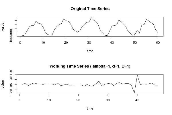
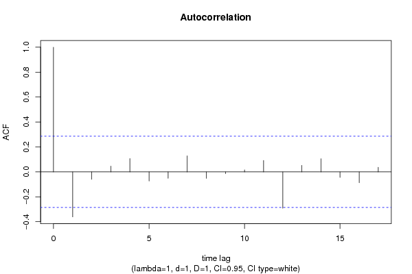
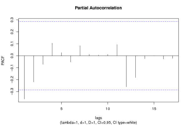
Title produced by software

(Partial) Autocorrelation Function

Date of computation

Tue, 06 Dec 2011 16:05:30 -0500

Cite this page as follows

Statistical Computations at FreeStatistics.org, Office for Research Development and Education, URL https://freestatistics.org/blog/index.php?v=date/2011/Dec/06/t1323205567cwhbpvmwtlnqwh9.htm/, Retrieved Mon, 29 Apr 2024 06:15:43 +0000

Statistical Computations at FreeStatistics.org, Office for Research Development and Education, URL https://freestatistics.org/blog/index.php?pk=151947, Retrieved Mon, 29 Apr 2024 06:15:43 +0000

QR Codes:

Paste this QR Code to cite your computation.

Original text written by user:

IsPrivate?

No (this computation is public)

User-defined keywords

Estimated Impact

Family? (F = Feedback message, R = changed R code, M = changed R Module, P = changed Parameters, D = changed Data)

-     [(Partial) Autocorrelation Function] [WS 9 Partial Auto...] [2011-12-06 20:53:20] [f5fdea4413921432bb019d1f20c4f2ec]
- R P     [(Partial) Autocorrelation Function] [WS 9 Partial Auto...] [2011-12-06 21:05:30] [6140f0163e532fc168d2f211324acd0a] [Current]
- RMP       [Spectral Analysis] [WS 9 Spectral Ana...] [2011-12-06 21:16:41] [f5fdea4413921432bb019d1f20c4f2ec] 
- R P         [Spectral Analysis] [WS 9 Spectral Ana...] [2011-12-06 21:35:07] [f5fdea4413921432bb019d1f20c4f2ec] 
-   P           [Spectral Analysis] [WS 9 Spectral Ana...] [2011-12-06 21:52:54] [f5fdea4413921432bb019d1f20c4f2ec] 
-   P             [Spectral Analysis] [WS 9 Spectral Ana...] [2011-12-16 12:23:12] [74be16979710d4c4e7c6647856088456] 
- RMP           [Variance Reduction Matrix] [WS 9 Variance Red...] [2011-12-06 22:12:11] [f5fdea4413921432bb019d1f20c4f2ec] 
- RMP           [Standard Deviation-Mean Plot] [Ws 9 Standard Dev...] [2011-12-06 22:25:52] [f5fdea4413921432bb019d1f20c4f2ec] 
- RMP           [ARIMA Backward Selection] [WS 9 ARIMA Backwa...] [2011-12-06 22:41:23] [f5fdea4413921432bb019d1f20c4f2ec] 
-   P           [Spectral Analysis] [WS 9 Spectral Ana...] [2011-12-16 11:57:04] [74be16979710d4c4e7c6647856088456] 
- R P         [Spectral Analysis] [WS 9 Spectral Ana...] [2011-12-16 11:52:18] [74be16979710d4c4e7c6647856088456] 

Feedback Forum

Post a new message

Dataseries X:

Download CSV

Histogram

Boxplots

Summary of computational transaction
Raw Input	view raw input (R code)
Raw Output	view raw output of R engine
Computing time	2 seconds
R Server	'Gwilym Jenkins' @ jenkins.wessa.net

\begin{tabular}{lllllllll}
\hline
Summary of computational transaction \tabularnewline
Raw Input & view raw input (R code)  \tabularnewline
Raw Output & view raw output of R engine  \tabularnewline
Computing time & 2 seconds \tabularnewline
R Server & 'Gwilym Jenkins' @ jenkins.wessa.net \tabularnewline
\hline
\end{tabular}
%Source: https://freestatistics.org/blog/index.php?pk=151947&T=0

[TABLE]
[ROW][C]Summary of computational transaction[/C][/ROW]
[ROW][C]Raw Input[/C][C]view raw input (R code) [/C][/ROW]
[ROW][C]Raw Output[/C][C]view raw output of R engine [/C][/ROW]
[ROW][C]Computing time[/C][C]2 seconds[/C][/ROW]
[ROW][C]R Server[/C][C]'Gwilym Jenkins' @ jenkins.wessa.net[/C][/ROW]
[/TABLE]
Source: https://freestatistics.org/blog/index.php?pk=151947&T=0

Globally Unique Identifier (entire table): ba.freestatistics.org/blog/index.php?pk=151947&T=0

As an alternative you can also use a QR Code:

The GUIDs for individual cells are displayed in the table below:

Summary of computational transaction
Raw Input	view raw input (R code)
Raw Output	view raw output of R engine
Computing time	2 seconds
R Server	'Gwilym Jenkins' @ jenkins.wessa.net

Autocorrelation Function
Time lag k	ACF(k)	T-STAT	P-value
1	-0.361157	-2.476	0.008473
2	-0.059843	-0.4103	0.341738
3	0.045975	0.3152	0.377007
4	0.106786	0.7321	0.233876
5	-0.073077	-0.501	0.309357
6	-0.051485	-0.353	0.362846
7	0.129131	0.8853	0.190257
8	-0.051983	-0.3564	0.361577
9	-0.01392	-0.0954	0.462189
10	0.015906	0.109	0.456815
11	0.09149	0.6272	0.266774
12	-0.291925	-2.0013	0.025574
13	0.052369	0.359	0.360593
14	0.105268	0.7217	0.237032
15	-0.044301	-0.3037	0.381343
16	-0.0872	-0.5978	0.276417
17	0.036657	0.2513	0.401335

\begin{tabular}{lllllllll}
\hline
Autocorrelation Function \tabularnewline
Time lag k & ACF(k) & T-STAT & P-value \tabularnewline
1 & -0.361157 & -2.476 & 0.008473 \tabularnewline
2 & -0.059843 & -0.4103 & 0.341738 \tabularnewline
3 & 0.045975 & 0.3152 & 0.377007 \tabularnewline
4 & 0.106786 & 0.7321 & 0.233876 \tabularnewline
5 & -0.073077 & -0.501 & 0.309357 \tabularnewline
6 & -0.051485 & -0.353 & 0.362846 \tabularnewline
7 & 0.129131 & 0.8853 & 0.190257 \tabularnewline
8 & -0.051983 & -0.3564 & 0.361577 \tabularnewline
9 & -0.01392 & -0.0954 & 0.462189 \tabularnewline
10 & 0.015906 & 0.109 & 0.456815 \tabularnewline
11 & 0.09149 & 0.6272 & 0.266774 \tabularnewline
12 & -0.291925 & -2.0013 & 0.025574 \tabularnewline
13 & 0.052369 & 0.359 & 0.360593 \tabularnewline
14 & 0.105268 & 0.7217 & 0.237032 \tabularnewline
15 & -0.044301 & -0.3037 & 0.381343 \tabularnewline
16 & -0.0872 & -0.5978 & 0.276417 \tabularnewline
17 & 0.036657 & 0.2513 & 0.401335 \tabularnewline
\hline
\end{tabular}
%Source: https://freestatistics.org/blog/index.php?pk=151947&T=1

[TABLE]
[ROW][C]Autocorrelation Function[/C][/ROW]
[ROW][C]Time lag k[/C][C]ACF(k)[/C][C]T-STAT[/C][C]P-value[/C][/ROW]
[ROW][C]1[/C][C]-0.361157[/C][C]-2.476[/C][C]0.008473[/C][/ROW]
[ROW][C]2[/C][C]-0.059843[/C][C]-0.4103[/C][C]0.341738[/C][/ROW]
[ROW][C]3[/C][C]0.045975[/C][C]0.3152[/C][C]0.377007[/C][/ROW]
[ROW][C]4[/C][C]0.106786[/C][C]0.7321[/C][C]0.233876[/C][/ROW]
[ROW][C]5[/C][C]-0.073077[/C][C]-0.501[/C][C]0.309357[/C][/ROW]
[ROW][C]6[/C][C]-0.051485[/C][C]-0.353[/C][C]0.362846[/C][/ROW]
[ROW][C]7[/C][C]0.129131[/C][C]0.8853[/C][C]0.190257[/C][/ROW]
[ROW][C]8[/C][C]-0.051983[/C][C]-0.3564[/C][C]0.361577[/C][/ROW]
[ROW][C]9[/C][C]-0.01392[/C][C]-0.0954[/C][C]0.462189[/C][/ROW]
[ROW][C]10[/C][C]0.015906[/C][C]0.109[/C][C]0.456815[/C][/ROW]
[ROW][C]11[/C][C]0.09149[/C][C]0.6272[/C][C]0.266774[/C][/ROW]
[ROW][C]12[/C][C]-0.291925[/C][C]-2.0013[/C][C]0.025574[/C][/ROW]
[ROW][C]13[/C][C]0.052369[/C][C]0.359[/C][C]0.360593[/C][/ROW]
[ROW][C]14[/C][C]0.105268[/C][C]0.7217[/C][C]0.237032[/C][/ROW]
[ROW][C]15[/C][C]-0.044301[/C][C]-0.3037[/C][C]0.381343[/C][/ROW]
[ROW][C]16[/C][C]-0.0872[/C][C]-0.5978[/C][C]0.276417[/C][/ROW]
[ROW][C]17[/C][C]0.036657[/C][C]0.2513[/C][C]0.401335[/C][/ROW]
[/TABLE]
Source: https://freestatistics.org/blog/index.php?pk=151947&T=1

Globally Unique Identifier (entire table): ba.freestatistics.org/blog/index.php?pk=151947&T=1

As an alternative you can also use a QR Code:

The GUIDs for individual cells are displayed in the table below:

Autocorrelation Function
Time lag k	ACF(k)	T-STAT	P-value
1	-0.361157	-2.476	0.008473
2	-0.059843	-0.4103	0.341738
3	0.045975	0.3152	0.377007
4	0.106786	0.7321	0.233876
5	-0.073077	-0.501	0.309357
6	-0.051485	-0.353	0.362846
7	0.129131	0.8853	0.190257
8	-0.051983	-0.3564	0.361577
9	-0.01392	-0.0954	0.462189
10	0.015906	0.109	0.456815
11	0.09149	0.6272	0.266774
12	-0.291925	-2.0013	0.025574
13	0.052369	0.359	0.360593
14	0.105268	0.7217	0.237032
15	-0.044301	-0.3037	0.381343
16	-0.0872	-0.5978	0.276417
17	0.036657	0.2513	0.401335

Partial Autocorrelation Function
Time lag k	PACF(k)	T-STAT	P-value
1	-0.361157	-2.476	0.008473
2	-0.218819	-1.5001	0.070132
3	-0.07174	-0.4918	0.312567
4	0.105444	0.7229	0.236666
5	0.026715	0.1832	0.427733
6	-0.052969	-0.3631	0.359066
7	0.084128	0.5767	0.28343
8	0.011637	0.0798	0.468376
9	0.006307	0.0432	0.482846
10	0.011429	0.0784	0.46894
11	0.092795	0.6362	0.263876
12	-0.259679	-1.7803	0.040748
13	-0.18217	-1.2489	0.108944
14	-0.02441	-0.1673	0.433907
15	0.001054	0.0072	0.497131
16	-0.027508	-0.1886	0.425615
17	-0.021455	-0.1471	0.441845

\begin{tabular}{lllllllll}
\hline
Partial Autocorrelation Function \tabularnewline
Time lag k & PACF(k) & T-STAT & P-value \tabularnewline
1 & -0.361157 & -2.476 & 0.008473 \tabularnewline
2 & -0.218819 & -1.5001 & 0.070132 \tabularnewline
3 & -0.07174 & -0.4918 & 0.312567 \tabularnewline
4 & 0.105444 & 0.7229 & 0.236666 \tabularnewline
5 & 0.026715 & 0.1832 & 0.427733 \tabularnewline
6 & -0.052969 & -0.3631 & 0.359066 \tabularnewline
7 & 0.084128 & 0.5767 & 0.28343 \tabularnewline
8 & 0.011637 & 0.0798 & 0.468376 \tabularnewline
9 & 0.006307 & 0.0432 & 0.482846 \tabularnewline
10 & 0.011429 & 0.0784 & 0.46894 \tabularnewline
11 & 0.092795 & 0.6362 & 0.263876 \tabularnewline
12 & -0.259679 & -1.7803 & 0.040748 \tabularnewline
13 & -0.18217 & -1.2489 & 0.108944 \tabularnewline
14 & -0.02441 & -0.1673 & 0.433907 \tabularnewline
15 & 0.001054 & 0.0072 & 0.497131 \tabularnewline
16 & -0.027508 & -0.1886 & 0.425615 \tabularnewline
17 & -0.021455 & -0.1471 & 0.441845 \tabularnewline
\hline
\end{tabular}
%Source: https://freestatistics.org/blog/index.php?pk=151947&T=2

[TABLE]
[ROW][C]Partial Autocorrelation Function[/C][/ROW]
[ROW][C]Time lag k[/C][C]PACF(k)[/C][C]T-STAT[/C][C]P-value[/C][/ROW]
[ROW][C]1[/C][C]-0.361157[/C][C]-2.476[/C][C]0.008473[/C][/ROW]
[ROW][C]2[/C][C]-0.218819[/C][C]-1.5001[/C][C]0.070132[/C][/ROW]
[ROW][C]3[/C][C]-0.07174[/C][C]-0.4918[/C][C]0.312567[/C][/ROW]
[ROW][C]4[/C][C]0.105444[/C][C]0.7229[/C][C]0.236666[/C][/ROW]
[ROW][C]5[/C][C]0.026715[/C][C]0.1832[/C][C]0.427733[/C][/ROW]
[ROW][C]6[/C][C]-0.052969[/C][C]-0.3631[/C][C]0.359066[/C][/ROW]
[ROW][C]7[/C][C]0.084128[/C][C]0.5767[/C][C]0.28343[/C][/ROW]
[ROW][C]8[/C][C]0.011637[/C][C]0.0798[/C][C]0.468376[/C][/ROW]
[ROW][C]9[/C][C]0.006307[/C][C]0.0432[/C][C]0.482846[/C][/ROW]
[ROW][C]10[/C][C]0.011429[/C][C]0.0784[/C][C]0.46894[/C][/ROW]
[ROW][C]11[/C][C]0.092795[/C][C]0.6362[/C][C]0.263876[/C][/ROW]
[ROW][C]12[/C][C]-0.259679[/C][C]-1.7803[/C][C]0.040748[/C][/ROW]
[ROW][C]13[/C][C]-0.18217[/C][C]-1.2489[/C][C]0.108944[/C][/ROW]
[ROW][C]14[/C][C]-0.02441[/C][C]-0.1673[/C][C]0.433907[/C][/ROW]
[ROW][C]15[/C][C]0.001054[/C][C]0.0072[/C][C]0.497131[/C][/ROW]
[ROW][C]16[/C][C]-0.027508[/C][C]-0.1886[/C][C]0.425615[/C][/ROW]
[ROW][C]17[/C][C]-0.021455[/C][C]-0.1471[/C][C]0.441845[/C][/ROW]
[/TABLE]
Source: https://freestatistics.org/blog/index.php?pk=151947&T=2

Globally Unique Identifier (entire table): ba.freestatistics.org/blog/index.php?pk=151947&T=2

As an alternative you can also use a QR Code:

The GUIDs for individual cells are displayed in the table below:

Partial Autocorrelation Function
Time lag k	PACF(k)	T-STAT	P-value
1	-0.361157	-2.476	0.008473
2	-0.218819	-1.5001	0.070132
3	-0.07174	-0.4918	0.312567
4	0.105444	0.7229	0.236666
5	0.026715	0.1832	0.427733
6	-0.052969	-0.3631	0.359066
7	0.084128	0.5767	0.28343
8	0.011637	0.0798	0.468376
9	0.006307	0.0432	0.482846
10	0.011429	0.0784	0.46894
11	0.092795	0.6362	0.263876
12	-0.259679	-1.7803	0.040748
13	-0.18217	-1.2489	0.108944
14	-0.02441	-0.1673	0.433907
15	0.001054	0.0072	0.497131
16	-0.027508	-0.1886	0.425615
17	-0.021455	-0.1471	0.441845

Figure 1

PNG link

Postscript link

PDF link

Figure 2

PNG link

Postscript link

PDF link

Figure 3

PNG link

Postscript link

PDF link

Parameters (Session):

par1 = Default ; par2 = 1 ; par3 = 1 ; par4 = 1 ; par5 = 12 ; par6 = White Noise ; par7 = 0.95 ;

Parameters (R input):

par1 = Default ; par2 = 1 ; par3 = 1 ; par4 = 1 ; par5 = 12 ; par6 = White Noise ; par7 = 0.95 ; par8 = ;

R code (references can be found in the software module):

if (par1 == 'Default') {
par1 = 10*log10(length(x))
} else {
par1 <- as.numeric(par1)
}
par2 <- as.numeric(par2)
par3 <- as.numeric(par3)
par4 <- as.numeric(par4)
par5 <- as.numeric(par5)
if (par6 == 'White Noise') par6 <- 'white' else par6 <- 'ma'
par7 <- as.numeric(par7)
if (par8 != '') par8 <- as.numeric(par8)
ox <- x
if (par8 == '') {
if (par2 == 0) {
x <- log(x)
} else {
x <- (x ^ par2 - 1) / par2
}
} else {
x <- log(x,base=par8)
}
if (par3 > 0) x <- diff(x,lag=1,difference=par3)
if (par4 > 0) x <- diff(x,lag=par5,difference=par4)
bitmap(file='picts.png')
op <- par(mfrow=c(2,1))
plot(ox,type='l',main='Original Time Series',xlab='time',ylab='value')
if (par8=='') {
mytitle <- paste('Working Time Series (lambda=',par2,', d=',par3,', D=',par4,')',sep='')
mysub <- paste('(lambda=',par2,', d=',par3,', D=',par4,', CI=', par7, ', CI type=',par6,')',sep='')
} else {
mytitle <- paste('Working Time Series (base=',par8,', d=',par3,', D=',par4,')',sep='')
mysub <- paste('(base=',par8,', d=',par3,', D=',par4,', CI=', par7, ', CI type=',par6,')',sep='')
}
plot(x,type='l', main=mytitle,xlab='time',ylab='value')
par(op)
dev.off()
bitmap(file='pic1.png')
racf <- acf(x, par1, main='Autocorrelation', xlab='time lag', ylab='ACF', ci.type=par6, ci=par7, sub=mysub)
dev.off()
bitmap(file='pic2.png')
rpacf <- pacf(x,par1,main='Partial Autocorrelation',xlab='lags',ylab='PACF',sub=mysub)
dev.off()
(myacf <- c(racf$acf))
(mypacf <- c(rpacf$acf))
lengthx <- length(x)
sqrtn <- sqrt(lengthx)
load(file='createtable')
a<-table.start()
a<-table.row.start(a)
a<-table.element(a,'Autocorrelation Function',4,TRUE)
a<-table.row.end(a)
a<-table.row.start(a)
a<-table.element(a,'Time lag k',header=TRUE)
a<-table.element(a,hyperlink('basics.htm','ACF(k)','click here for more information about the Autocorrelation Function'),header=TRUE)
a<-table.element(a,'T-STAT',header=TRUE)
a<-table.element(a,'P-value',header=TRUE)
a<-table.row.end(a)
for (i in 2:(par1+1)) {
a<-table.row.start(a)
a<-table.element(a,i-1,header=TRUE)
a<-table.element(a,round(myacf[i],6))
mytstat <- myacf[i]*sqrtn
a<-table.element(a,round(mytstat,4))
a<-table.element(a,round(1-pt(abs(mytstat),lengthx),6))
a<-table.row.end(a)
}
a<-table.end(a)
table.save(a,file='mytable.tab')
a<-table.start()
a<-table.row.start(a)
a<-table.element(a,'Partial Autocorrelation Function',4,TRUE)
a<-table.row.end(a)
a<-table.row.start(a)
a<-table.element(a,'Time lag k',header=TRUE)
a<-table.element(a,hyperlink('basics.htm','PACF(k)','click here for more information about the Partial Autocorrelation Function'),header=TRUE)
a<-table.element(a,'T-STAT',header=TRUE)
a<-table.element(a,'P-value',header=TRUE)
a<-table.row.end(a)
for (i in 1:par1) {
a<-table.row.start(a)
a<-table.element(a,i,header=TRUE)
a<-table.element(a,round(mypacf[i],6))
mytstat <- mypacf[i]*sqrtn
a<-table.element(a,round(mytstat,4))
a<-table.element(a,round(1-pt(abs(mytstat),lengthx),6))
a<-table.row.end(a)
}
a<-table.end(a)
table.save(a,file='mytable1.tab')

Free Statistics

Description of Statistical Computation

Tree of Dependent Computations

Dataset

Tables (Output of Computation)

Figures (Output of Computation)

Input Parameters & R Code