Repository of Reproducible Computations

Free Statistics

of Irreproducible Research!

Author's title

Author

*The author of this computation has been verified*

R Software Module

rwasp_autocorrelation.wasp

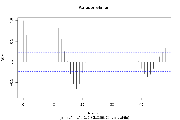
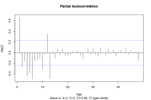
Title produced by software

(Partial) Autocorrelation Function

Date of computation

Tue, 06 Dec 2011 14:34:16 -0500

Cite this page as follows

Statistical Computations at FreeStatistics.org, Office for Research Development and Education, URL https://freestatistics.org/blog/index.php?v=date/2011/Dec/06/t1323200084ghzrdmx71sjq5ej.htm/, Retrieved Mon, 29 Apr 2024 03:29:03 +0000

Statistical Computations at FreeStatistics.org, Office for Research Development and Education, URL https://freestatistics.org/blog/index.php?pk=151830, Retrieved Mon, 29 Apr 2024 03:29:03 +0000

QR Codes:

Paste this QR Code to cite your computation.

Original text written by user:

IsPrivate?

No (this computation is public)

User-defined keywords

Estimated Impact

116

Family? (F = Feedback message, R = changed R code, M = changed R Module, P = changed Parameters, D = changed Data)

-     [Univariate Explorative Data Analysis] [Run Sequence gebo...] [2008-12-12 13:32:37] [76963dc1903f0f612b6153510a3818cf]
- R  D  [Univariate Explorative Data Analysis] [Run Sequence gebo...] [2008-12-17 12:14:40] [76963dc1903f0f612b6153510a3818cf]
-         [Univariate Explorative Data Analysis] [Run Sequence Plot...] [2008-12-22 18:19:51] [1ce0d16c8f4225c977b42c8fa93bc163]
- RMP       [Univariate Data Series] [Identifying Integ...] [2009-11-22 12:08:06] [b98453cac15ba1066b407e146608df68]
- RMP         [(Partial) Autocorrelation Function] [Births] [2010-11-29 09:36:27] [b98453cac15ba1066b407e146608df68]
F R PD          [(Partial) Autocorrelation Function] [autocorrelatiefun...] [2010-12-02 19:51:36] [97ad38b1c3b35a5feca8b85f7bc7b3ff]
- R P             [(Partial) Autocorrelation Function] [] [2011-12-04 12:40:04] [9401a40688cf36283be626153bc5a38b]
- R                   [(Partial) Autocorrelation Function] [WS9.2] [2011-12-06 19:34:16] [7c363341293f6644b8647ab9153ed4f7] [Current]

Feedback Forum

Post a new message

Dataseries X:

Download CSV

Histogram

Boxplots

Summary of computational transaction
Raw Input	view raw input (R code)
Raw Output	view raw output of R engine
Computing time	2 seconds
R Server	'George Udny Yule' @ yule.wessa.net

\begin{tabular}{lllllllll}
\hline
Summary of computational transaction \tabularnewline
Raw Input & view raw input (R code)  \tabularnewline
Raw Output & view raw output of R engine  \tabularnewline
Computing time & 2 seconds \tabularnewline
R Server & 'George Udny Yule' @ yule.wessa.net \tabularnewline
\hline
\end{tabular}
%Source: https://freestatistics.org/blog/index.php?pk=151830&T=0

[TABLE]
[ROW][C]Summary of computational transaction[/C][/ROW]
[ROW][C]Raw Input[/C][C]view raw input (R code) [/C][/ROW]
[ROW][C]Raw Output[/C][C]view raw output of R engine [/C][/ROW]
[ROW][C]Computing time[/C][C]2 seconds[/C][/ROW]
[ROW][C]R Server[/C][C]'George Udny Yule' @ yule.wessa.net[/C][/ROW]
[/TABLE]
Source: https://freestatistics.org/blog/index.php?pk=151830&T=0

Globally Unique Identifier (entire table): ba.freestatistics.org/blog/index.php?pk=151830&T=0

As an alternative you can also use a QR Code:

The GUIDs for individual cells are displayed in the table below:

Summary of computational transaction
Raw Input	view raw input (R code)
Raw Output	view raw output of R engine
Computing time	2 seconds
R Server	'George Udny Yule' @ yule.wessa.net

Autocorrelation Function
Time lag k	ACF(k)	T-STAT	P-value
1	0.663664	5.6314	0
2	0.294956	2.5028	0.007296
3	-0.006926	-0.0588	0.476649
4	-0.367116	-3.1151	0.00132
5	-0.652937	-5.5404	0
6	-0.799623	-6.785	0
7	-0.639245	-5.4242	0
8	-0.315998	-2.6813	0.004543
9	0.010407	0.0883	0.464939
10	0.290081	2.4614	0.008118
11	0.587897	4.9885	2e-06
12	0.821917	6.9742	0
13	0.554832	4.7079	6e-06
14	0.25402	2.1554	0.017236
15	0.004818	0.0409	0.483753
16	-0.292861	-2.485	0.00764
17	-0.525597	-4.4598	1.5e-05
18	-0.650951	-5.5235	0
19	-0.525294	-4.4573	1.5e-05
20	-0.259283	-2.2001	0.015505
21	-0.009723	-0.0825	0.467237
22	0.227197	1.9278	0.02891
23	0.470847	3.9953	7.7e-05
24	0.65056	5.5202	0
25	0.447939	3.8009	0.00015
26	0.196934	1.671	0.049527
27	0.008929	0.0758	0.46991
28	-0.210636	-1.7873	0.039048
29	-0.406749	-3.4514	0.000469
30	-0.502798	-4.2664	3e-05
31	-0.408352	-3.465	0.000449
32	-0.211116	-1.7914	0.038718
33	-0.007342	-0.0623	0.47525
34	0.172364	1.4626	0.07397
35	0.342873	2.9094	0.002407
36	0.494991	4.2001	3.8e-05
37	0.342068	2.9025	0.002455
38	0.153597	1.3033	0.098311
39	0.013388	0.1136	0.454935
40	-0.157824	-1.3392	0.092362
41	-0.296415	-2.5152	0.007065
42	-0.370952	-3.1476	0.001198
43	-0.299961	-2.5453	0.006531
44	-0.159051	-1.3496	0.090688
45	-0.005336	-0.0453	0.482004
46	0.126831	1.0762	0.142717
47	0.237767	2.0175	0.023685
48	0.336241	2.8531	0.002824

\begin{tabular}{lllllllll}
\hline
Autocorrelation Function \tabularnewline
Time lag k & ACF(k) & T-STAT & P-value \tabularnewline
1 & 0.663664 & 5.6314 & 0 \tabularnewline
2 & 0.294956 & 2.5028 & 0.007296 \tabularnewline
3 & -0.006926 & -0.0588 & 0.476649 \tabularnewline
4 & -0.367116 & -3.1151 & 0.00132 \tabularnewline
5 & -0.652937 & -5.5404 & 0 \tabularnewline
6 & -0.799623 & -6.785 & 0 \tabularnewline
7 & -0.639245 & -5.4242 & 0 \tabularnewline
8 & -0.315998 & -2.6813 & 0.004543 \tabularnewline
9 & 0.010407 & 0.0883 & 0.464939 \tabularnewline
10 & 0.290081 & 2.4614 & 0.008118 \tabularnewline
11 & 0.587897 & 4.9885 & 2e-06 \tabularnewline
12 & 0.821917 & 6.9742 & 0 \tabularnewline
13 & 0.554832 & 4.7079 & 6e-06 \tabularnewline
14 & 0.25402 & 2.1554 & 0.017236 \tabularnewline
15 & 0.004818 & 0.0409 & 0.483753 \tabularnewline
16 & -0.292861 & -2.485 & 0.00764 \tabularnewline
17 & -0.525597 & -4.4598 & 1.5e-05 \tabularnewline
18 & -0.650951 & -5.5235 & 0 \tabularnewline
19 & -0.525294 & -4.4573 & 1.5e-05 \tabularnewline
20 & -0.259283 & -2.2001 & 0.015505 \tabularnewline
21 & -0.009723 & -0.0825 & 0.467237 \tabularnewline
22 & 0.227197 & 1.9278 & 0.02891 \tabularnewline
23 & 0.470847 & 3.9953 & 7.7e-05 \tabularnewline
24 & 0.65056 & 5.5202 & 0 \tabularnewline
25 & 0.447939 & 3.8009 & 0.00015 \tabularnewline
26 & 0.196934 & 1.671 & 0.049527 \tabularnewline
27 & 0.008929 & 0.0758 & 0.46991 \tabularnewline
28 & -0.210636 & -1.7873 & 0.039048 \tabularnewline
29 & -0.406749 & -3.4514 & 0.000469 \tabularnewline
30 & -0.502798 & -4.2664 & 3e-05 \tabularnewline
31 & -0.408352 & -3.465 & 0.000449 \tabularnewline
32 & -0.211116 & -1.7914 & 0.038718 \tabularnewline
33 & -0.007342 & -0.0623 & 0.47525 \tabularnewline
34 & 0.172364 & 1.4626 & 0.07397 \tabularnewline
35 & 0.342873 & 2.9094 & 0.002407 \tabularnewline
36 & 0.494991 & 4.2001 & 3.8e-05 \tabularnewline
37 & 0.342068 & 2.9025 & 0.002455 \tabularnewline
38 & 0.153597 & 1.3033 & 0.098311 \tabularnewline
39 & 0.013388 & 0.1136 & 0.454935 \tabularnewline
40 & -0.157824 & -1.3392 & 0.092362 \tabularnewline
41 & -0.296415 & -2.5152 & 0.007065 \tabularnewline
42 & -0.370952 & -3.1476 & 0.001198 \tabularnewline
43 & -0.299961 & -2.5453 & 0.006531 \tabularnewline
44 & -0.159051 & -1.3496 & 0.090688 \tabularnewline
45 & -0.005336 & -0.0453 & 0.482004 \tabularnewline
46 & 0.126831 & 1.0762 & 0.142717 \tabularnewline
47 & 0.237767 & 2.0175 & 0.023685 \tabularnewline
48 & 0.336241 & 2.8531 & 0.002824 \tabularnewline
\hline
\end{tabular}
%Source: https://freestatistics.org/blog/index.php?pk=151830&T=1

[TABLE]
[ROW][C]Autocorrelation Function[/C][/ROW]
[ROW][C]Time lag k[/C][C]ACF(k)[/C][C]T-STAT[/C][C]P-value[/C][/ROW]
[ROW][C]1[/C][C]0.663664[/C][C]5.6314[/C][C]0[/C][/ROW]
[ROW][C]2[/C][C]0.294956[/C][C]2.5028[/C][C]0.007296[/C][/ROW]
[ROW][C]3[/C][C]-0.006926[/C][C]-0.0588[/C][C]0.476649[/C][/ROW]
[ROW][C]4[/C][C]-0.367116[/C][C]-3.1151[/C][C]0.00132[/C][/ROW]
[ROW][C]5[/C][C]-0.652937[/C][C]-5.5404[/C][C]0[/C][/ROW]
[ROW][C]6[/C][C]-0.799623[/C][C]-6.785[/C][C]0[/C][/ROW]
[ROW][C]7[/C][C]-0.639245[/C][C]-5.4242[/C][C]0[/C][/ROW]
[ROW][C]8[/C][C]-0.315998[/C][C]-2.6813[/C][C]0.004543[/C][/ROW]
[ROW][C]9[/C][C]0.010407[/C][C]0.0883[/C][C]0.464939[/C][/ROW]
[ROW][C]10[/C][C]0.290081[/C][C]2.4614[/C][C]0.008118[/C][/ROW]
[ROW][C]11[/C][C]0.587897[/C][C]4.9885[/C][C]2e-06[/C][/ROW]
[ROW][C]12[/C][C]0.821917[/C][C]6.9742[/C][C]0[/C][/ROW]
[ROW][C]13[/C][C]0.554832[/C][C]4.7079[/C][C]6e-06[/C][/ROW]
[ROW][C]14[/C][C]0.25402[/C][C]2.1554[/C][C]0.017236[/C][/ROW]
[ROW][C]15[/C][C]0.004818[/C][C]0.0409[/C][C]0.483753[/C][/ROW]
[ROW][C]16[/C][C]-0.292861[/C][C]-2.485[/C][C]0.00764[/C][/ROW]
[ROW][C]17[/C][C]-0.525597[/C][C]-4.4598[/C][C]1.5e-05[/C][/ROW]
[ROW][C]18[/C][C]-0.650951[/C][C]-5.5235[/C][C]0[/C][/ROW]
[ROW][C]19[/C][C]-0.525294[/C][C]-4.4573[/C][C]1.5e-05[/C][/ROW]
[ROW][C]20[/C][C]-0.259283[/C][C]-2.2001[/C][C]0.015505[/C][/ROW]
[ROW][C]21[/C][C]-0.009723[/C][C]-0.0825[/C][C]0.467237[/C][/ROW]
[ROW][C]22[/C][C]0.227197[/C][C]1.9278[/C][C]0.02891[/C][/ROW]
[ROW][C]23[/C][C]0.470847[/C][C]3.9953[/C][C]7.7e-05[/C][/ROW]
[ROW][C]24[/C][C]0.65056[/C][C]5.5202[/C][C]0[/C][/ROW]
[ROW][C]25[/C][C]0.447939[/C][C]3.8009[/C][C]0.00015[/C][/ROW]
[ROW][C]26[/C][C]0.196934[/C][C]1.671[/C][C]0.049527[/C][/ROW]
[ROW][C]27[/C][C]0.008929[/C][C]0.0758[/C][C]0.46991[/C][/ROW]
[ROW][C]28[/C][C]-0.210636[/C][C]-1.7873[/C][C]0.039048[/C][/ROW]
[ROW][C]29[/C][C]-0.406749[/C][C]-3.4514[/C][C]0.000469[/C][/ROW]
[ROW][C]30[/C][C]-0.502798[/C][C]-4.2664[/C][C]3e-05[/C][/ROW]
[ROW][C]31[/C][C]-0.408352[/C][C]-3.465[/C][C]0.000449[/C][/ROW]
[ROW][C]32[/C][C]-0.211116[/C][C]-1.7914[/C][C]0.038718[/C][/ROW]
[ROW][C]33[/C][C]-0.007342[/C][C]-0.0623[/C][C]0.47525[/C][/ROW]
[ROW][C]34[/C][C]0.172364[/C][C]1.4626[/C][C]0.07397[/C][/ROW]
[ROW][C]35[/C][C]0.342873[/C][C]2.9094[/C][C]0.002407[/C][/ROW]
[ROW][C]36[/C][C]0.494991[/C][C]4.2001[/C][C]3.8e-05[/C][/ROW]
[ROW][C]37[/C][C]0.342068[/C][C]2.9025[/C][C]0.002455[/C][/ROW]
[ROW][C]38[/C][C]0.153597[/C][C]1.3033[/C][C]0.098311[/C][/ROW]
[ROW][C]39[/C][C]0.013388[/C][C]0.1136[/C][C]0.454935[/C][/ROW]
[ROW][C]40[/C][C]-0.157824[/C][C]-1.3392[/C][C]0.092362[/C][/ROW]
[ROW][C]41[/C][C]-0.296415[/C][C]-2.5152[/C][C]0.007065[/C][/ROW]
[ROW][C]42[/C][C]-0.370952[/C][C]-3.1476[/C][C]0.001198[/C][/ROW]
[ROW][C]43[/C][C]-0.299961[/C][C]-2.5453[/C][C]0.006531[/C][/ROW]
[ROW][C]44[/C][C]-0.159051[/C][C]-1.3496[/C][C]0.090688[/C][/ROW]
[ROW][C]45[/C][C]-0.005336[/C][C]-0.0453[/C][C]0.482004[/C][/ROW]
[ROW][C]46[/C][C]0.126831[/C][C]1.0762[/C][C]0.142717[/C][/ROW]
[ROW][C]47[/C][C]0.237767[/C][C]2.0175[/C][C]0.023685[/C][/ROW]
[ROW][C]48[/C][C]0.336241[/C][C]2.8531[/C][C]0.002824[/C][/ROW]
[/TABLE]
Source: https://freestatistics.org/blog/index.php?pk=151830&T=1

Globally Unique Identifier (entire table): ba.freestatistics.org/blog/index.php?pk=151830&T=1

As an alternative you can also use a QR Code:

The GUIDs for individual cells are displayed in the table below:

Autocorrelation Function
Time lag k	ACF(k)	T-STAT	P-value
1	0.663664	5.6314	0
2	0.294956	2.5028	0.007296
3	-0.006926	-0.0588	0.476649
4	-0.367116	-3.1151	0.00132
5	-0.652937	-5.5404	0
6	-0.799623	-6.785	0
7	-0.639245	-5.4242	0
8	-0.315998	-2.6813	0.004543
9	0.010407	0.0883	0.464939
10	0.290081	2.4614	0.008118
11	0.587897	4.9885	2e-06
12	0.821917	6.9742	0
13	0.554832	4.7079	6e-06
14	0.25402	2.1554	0.017236
15	0.004818	0.0409	0.483753
16	-0.292861	-2.485	0.00764
17	-0.525597	-4.4598	1.5e-05
18	-0.650951	-5.5235	0
19	-0.525294	-4.4573	1.5e-05
20	-0.259283	-2.2001	0.015505
21	-0.009723	-0.0825	0.467237
22	0.227197	1.9278	0.02891
23	0.470847	3.9953	7.7e-05
24	0.65056	5.5202	0
25	0.447939	3.8009	0.00015
26	0.196934	1.671	0.049527
27	0.008929	0.0758	0.46991
28	-0.210636	-1.7873	0.039048
29	-0.406749	-3.4514	0.000469
30	-0.502798	-4.2664	3e-05
31	-0.408352	-3.465	0.000449
32	-0.211116	-1.7914	0.038718
33	-0.007342	-0.0623	0.47525
34	0.172364	1.4626	0.07397
35	0.342873	2.9094	0.002407
36	0.494991	4.2001	3.8e-05
37	0.342068	2.9025	0.002455
38	0.153597	1.3033	0.098311
39	0.013388	0.1136	0.454935
40	-0.157824	-1.3392	0.092362
41	-0.296415	-2.5152	0.007065
42	-0.370952	-3.1476	0.001198
43	-0.299961	-2.5453	0.006531
44	-0.159051	-1.3496	0.090688
45	-0.005336	-0.0453	0.482004
46	0.126831	1.0762	0.142717
47	0.237767	2.0175	0.023685
48	0.336241	2.8531	0.002824

Partial Autocorrelation Function
Time lag k	PACF(k)	T-STAT	P-value
1	0.663664	5.6314	0
2	-0.26002	-2.2063	0.015275
3	-0.155279	-1.3176	0.09591
4	-0.432408	-3.6691	0.000232
5	-0.375505	-3.1863	0.001066
6	-0.493265	-4.1855	4e-05
7	-0.154978	-1.315	0.096335
8	-0.12642	-1.0727	0.143492
9	-0.111026	-0.9421	0.17465
10	-0.310509	-2.6348	0.005151
11	-0.026259	-0.2228	0.412156
12	0.35077	2.9764	0.001985
13	-0.479442	-4.0682	6e-05
14	-0.022431	-0.1903	0.424793
15	-0.099268	-0.8423	0.2012
16	0.078736	0.6681	0.253103
17	-0.046605	-0.3955	0.346839
18	0.071079	0.6031	0.274162
19	-0.055801	-0.4735	0.318648
20	-0.052817	-0.4482	0.327688
21	-0.037288	-0.3164	0.376306
22	0.028142	0.2388	0.405972
23	0.01453	0.1233	0.451111
24	0.042545	0.361	0.359575
25	-0.049855	-0.423	0.336765
26	-0.115253	-0.978	0.165685
27	0.000164	0.0014	0.499445
28	0.070936	0.6019	0.274562
29	-0.030382	-0.2578	0.398647
30	0.080779	0.6854	0.247637
31	-0.032805	-0.2784	0.390766
32	-0.060479	-0.5132	0.304697
33	0.097339	0.826	0.20578
34	0.002103	0.0178	0.492905
35	-0.046556	-0.395	0.346992
36	0.074435	0.6316	0.264825
37	-0.019168	-0.1626	0.435627
38	0.057354	0.4867	0.313988
39	-0.064765	-0.5495	0.292166
40	0.013841	0.1174	0.453417
41	0.052492	0.4454	0.328681
42	0.006546	0.0555	0.477928
43	0.087461	0.7421	0.230212
44	-0.025372	-0.2153	0.415074
45	0.043845	0.372	0.35548
46	0.008556	0.0726	0.471164
47	0.023043	0.1955	0.422766
48	-0.148956	-1.2639	0.105166

\begin{tabular}{lllllllll}
\hline
Partial Autocorrelation Function \tabularnewline
Time lag k & PACF(k) & T-STAT & P-value \tabularnewline
1 & 0.663664 & 5.6314 & 0 \tabularnewline
2 & -0.26002 & -2.2063 & 0.015275 \tabularnewline
3 & -0.155279 & -1.3176 & 0.09591 \tabularnewline
4 & -0.432408 & -3.6691 & 0.000232 \tabularnewline
5 & -0.375505 & -3.1863 & 0.001066 \tabularnewline
6 & -0.493265 & -4.1855 & 4e-05 \tabularnewline
7 & -0.154978 & -1.315 & 0.096335 \tabularnewline
8 & -0.12642 & -1.0727 & 0.143492 \tabularnewline
9 & -0.111026 & -0.9421 & 0.17465 \tabularnewline
10 & -0.310509 & -2.6348 & 0.005151 \tabularnewline
11 & -0.026259 & -0.2228 & 0.412156 \tabularnewline
12 & 0.35077 & 2.9764 & 0.001985 \tabularnewline
13 & -0.479442 & -4.0682 & 6e-05 \tabularnewline
14 & -0.022431 & -0.1903 & 0.424793 \tabularnewline
15 & -0.099268 & -0.8423 & 0.2012 \tabularnewline
16 & 0.078736 & 0.6681 & 0.253103 \tabularnewline
17 & -0.046605 & -0.3955 & 0.346839 \tabularnewline
18 & 0.071079 & 0.6031 & 0.274162 \tabularnewline
19 & -0.055801 & -0.4735 & 0.318648 \tabularnewline
20 & -0.052817 & -0.4482 & 0.327688 \tabularnewline
21 & -0.037288 & -0.3164 & 0.376306 \tabularnewline
22 & 0.028142 & 0.2388 & 0.405972 \tabularnewline
23 & 0.01453 & 0.1233 & 0.451111 \tabularnewline
24 & 0.042545 & 0.361 & 0.359575 \tabularnewline
25 & -0.049855 & -0.423 & 0.336765 \tabularnewline
26 & -0.115253 & -0.978 & 0.165685 \tabularnewline
27 & 0.000164 & 0.0014 & 0.499445 \tabularnewline
28 & 0.070936 & 0.6019 & 0.274562 \tabularnewline
29 & -0.030382 & -0.2578 & 0.398647 \tabularnewline
30 & 0.080779 & 0.6854 & 0.247637 \tabularnewline
31 & -0.032805 & -0.2784 & 0.390766 \tabularnewline
32 & -0.060479 & -0.5132 & 0.304697 \tabularnewline
33 & 0.097339 & 0.826 & 0.20578 \tabularnewline
34 & 0.002103 & 0.0178 & 0.492905 \tabularnewline
35 & -0.046556 & -0.395 & 0.346992 \tabularnewline
36 & 0.074435 & 0.6316 & 0.264825 \tabularnewline
37 & -0.019168 & -0.1626 & 0.435627 \tabularnewline
38 & 0.057354 & 0.4867 & 0.313988 \tabularnewline
39 & -0.064765 & -0.5495 & 0.292166 \tabularnewline
40 & 0.013841 & 0.1174 & 0.453417 \tabularnewline
41 & 0.052492 & 0.4454 & 0.328681 \tabularnewline
42 & 0.006546 & 0.0555 & 0.477928 \tabularnewline
43 & 0.087461 & 0.7421 & 0.230212 \tabularnewline
44 & -0.025372 & -0.2153 & 0.415074 \tabularnewline
45 & 0.043845 & 0.372 & 0.35548 \tabularnewline
46 & 0.008556 & 0.0726 & 0.471164 \tabularnewline
47 & 0.023043 & 0.1955 & 0.422766 \tabularnewline
48 & -0.148956 & -1.2639 & 0.105166 \tabularnewline
\hline
\end{tabular}
%Source: https://freestatistics.org/blog/index.php?pk=151830&T=2

[TABLE]
[ROW][C]Partial Autocorrelation Function[/C][/ROW]
[ROW][C]Time lag k[/C][C]PACF(k)[/C][C]T-STAT[/C][C]P-value[/C][/ROW]
[ROW][C]1[/C][C]0.663664[/C][C]5.6314[/C][C]0[/C][/ROW]
[ROW][C]2[/C][C]-0.26002[/C][C]-2.2063[/C][C]0.015275[/C][/ROW]
[ROW][C]3[/C][C]-0.155279[/C][C]-1.3176[/C][C]0.09591[/C][/ROW]
[ROW][C]4[/C][C]-0.432408[/C][C]-3.6691[/C][C]0.000232[/C][/ROW]
[ROW][C]5[/C][C]-0.375505[/C][C]-3.1863[/C][C]0.001066[/C][/ROW]
[ROW][C]6[/C][C]-0.493265[/C][C]-4.1855[/C][C]4e-05[/C][/ROW]
[ROW][C]7[/C][C]-0.154978[/C][C]-1.315[/C][C]0.096335[/C][/ROW]
[ROW][C]8[/C][C]-0.12642[/C][C]-1.0727[/C][C]0.143492[/C][/ROW]
[ROW][C]9[/C][C]-0.111026[/C][C]-0.9421[/C][C]0.17465[/C][/ROW]
[ROW][C]10[/C][C]-0.310509[/C][C]-2.6348[/C][C]0.005151[/C][/ROW]
[ROW][C]11[/C][C]-0.026259[/C][C]-0.2228[/C][C]0.412156[/C][/ROW]
[ROW][C]12[/C][C]0.35077[/C][C]2.9764[/C][C]0.001985[/C][/ROW]
[ROW][C]13[/C][C]-0.479442[/C][C]-4.0682[/C][C]6e-05[/C][/ROW]
[ROW][C]14[/C][C]-0.022431[/C][C]-0.1903[/C][C]0.424793[/C][/ROW]
[ROW][C]15[/C][C]-0.099268[/C][C]-0.8423[/C][C]0.2012[/C][/ROW]
[ROW][C]16[/C][C]0.078736[/C][C]0.6681[/C][C]0.253103[/C][/ROW]
[ROW][C]17[/C][C]-0.046605[/C][C]-0.3955[/C][C]0.346839[/C][/ROW]
[ROW][C]18[/C][C]0.071079[/C][C]0.6031[/C][C]0.274162[/C][/ROW]
[ROW][C]19[/C][C]-0.055801[/C][C]-0.4735[/C][C]0.318648[/C][/ROW]
[ROW][C]20[/C][C]-0.052817[/C][C]-0.4482[/C][C]0.327688[/C][/ROW]
[ROW][C]21[/C][C]-0.037288[/C][C]-0.3164[/C][C]0.376306[/C][/ROW]
[ROW][C]22[/C][C]0.028142[/C][C]0.2388[/C][C]0.405972[/C][/ROW]
[ROW][C]23[/C][C]0.01453[/C][C]0.1233[/C][C]0.451111[/C][/ROW]
[ROW][C]24[/C][C]0.042545[/C][C]0.361[/C][C]0.359575[/C][/ROW]
[ROW][C]25[/C][C]-0.049855[/C][C]-0.423[/C][C]0.336765[/C][/ROW]
[ROW][C]26[/C][C]-0.115253[/C][C]-0.978[/C][C]0.165685[/C][/ROW]
[ROW][C]27[/C][C]0.000164[/C][C]0.0014[/C][C]0.499445[/C][/ROW]
[ROW][C]28[/C][C]0.070936[/C][C]0.6019[/C][C]0.274562[/C][/ROW]
[ROW][C]29[/C][C]-0.030382[/C][C]-0.2578[/C][C]0.398647[/C][/ROW]
[ROW][C]30[/C][C]0.080779[/C][C]0.6854[/C][C]0.247637[/C][/ROW]
[ROW][C]31[/C][C]-0.032805[/C][C]-0.2784[/C][C]0.390766[/C][/ROW]
[ROW][C]32[/C][C]-0.060479[/C][C]-0.5132[/C][C]0.304697[/C][/ROW]
[ROW][C]33[/C][C]0.097339[/C][C]0.826[/C][C]0.20578[/C][/ROW]
[ROW][C]34[/C][C]0.002103[/C][C]0.0178[/C][C]0.492905[/C][/ROW]
[ROW][C]35[/C][C]-0.046556[/C][C]-0.395[/C][C]0.346992[/C][/ROW]
[ROW][C]36[/C][C]0.074435[/C][C]0.6316[/C][C]0.264825[/C][/ROW]
[ROW][C]37[/C][C]-0.019168[/C][C]-0.1626[/C][C]0.435627[/C][/ROW]
[ROW][C]38[/C][C]0.057354[/C][C]0.4867[/C][C]0.313988[/C][/ROW]
[ROW][C]39[/C][C]-0.064765[/C][C]-0.5495[/C][C]0.292166[/C][/ROW]
[ROW][C]40[/C][C]0.013841[/C][C]0.1174[/C][C]0.453417[/C][/ROW]
[ROW][C]41[/C][C]0.052492[/C][C]0.4454[/C][C]0.328681[/C][/ROW]
[ROW][C]42[/C][C]0.006546[/C][C]0.0555[/C][C]0.477928[/C][/ROW]
[ROW][C]43[/C][C]0.087461[/C][C]0.7421[/C][C]0.230212[/C][/ROW]
[ROW][C]44[/C][C]-0.025372[/C][C]-0.2153[/C][C]0.415074[/C][/ROW]
[ROW][C]45[/C][C]0.043845[/C][C]0.372[/C][C]0.35548[/C][/ROW]
[ROW][C]46[/C][C]0.008556[/C][C]0.0726[/C][C]0.471164[/C][/ROW]
[ROW][C]47[/C][C]0.023043[/C][C]0.1955[/C][C]0.422766[/C][/ROW]
[ROW][C]48[/C][C]-0.148956[/C][C]-1.2639[/C][C]0.105166[/C][/ROW]
[/TABLE]
Source: https://freestatistics.org/blog/index.php?pk=151830&T=2

Globally Unique Identifier (entire table): ba.freestatistics.org/blog/index.php?pk=151830&T=2

As an alternative you can also use a QR Code:

The GUIDs for individual cells are displayed in the table below:

Partial Autocorrelation Function
Time lag k	PACF(k)	T-STAT	P-value
1	0.663664	5.6314	0
2	-0.26002	-2.2063	0.015275
3	-0.155279	-1.3176	0.09591
4	-0.432408	-3.6691	0.000232
5	-0.375505	-3.1863	0.001066
6	-0.493265	-4.1855	4e-05
7	-0.154978	-1.315	0.096335
8	-0.12642	-1.0727	0.143492
9	-0.111026	-0.9421	0.17465
10	-0.310509	-2.6348	0.005151
11	-0.026259	-0.2228	0.412156
12	0.35077	2.9764	0.001985
13	-0.479442	-4.0682	6e-05
14	-0.022431	-0.1903	0.424793
15	-0.099268	-0.8423	0.2012
16	0.078736	0.6681	0.253103
17	-0.046605	-0.3955	0.346839
18	0.071079	0.6031	0.274162
19	-0.055801	-0.4735	0.318648
20	-0.052817	-0.4482	0.327688
21	-0.037288	-0.3164	0.376306
22	0.028142	0.2388	0.405972
23	0.01453	0.1233	0.451111
24	0.042545	0.361	0.359575
25	-0.049855	-0.423	0.336765
26	-0.115253	-0.978	0.165685
27	0.000164	0.0014	0.499445
28	0.070936	0.6019	0.274562
29	-0.030382	-0.2578	0.398647
30	0.080779	0.6854	0.247637
31	-0.032805	-0.2784	0.390766
32	-0.060479	-0.5132	0.304697
33	0.097339	0.826	0.20578
34	0.002103	0.0178	0.492905
35	-0.046556	-0.395	0.346992
36	0.074435	0.6316	0.264825
37	-0.019168	-0.1626	0.435627
38	0.057354	0.4867	0.313988
39	-0.064765	-0.5495	0.292166
40	0.013841	0.1174	0.453417
41	0.052492	0.4454	0.328681
42	0.006546	0.0555	0.477928
43	0.087461	0.7421	0.230212
44	-0.025372	-0.2153	0.415074
45	0.043845	0.372	0.35548
46	0.008556	0.0726	0.471164
47	0.023043	0.1955	0.422766
48	-0.148956	-1.2639	0.105166

Figure 1

PNG link

Postscript link

PDF link

Figure 2

PNG link

Postscript link

PDF link

Figure 3

PNG link

Postscript link

PDF link

Parameters (Session):

par1 = 48 ; par2 = 1 ; par3 = 0 ; par4 = 0 ; par5 = 12 ; par6 = White Noise ; par7 = 0.95 ; par8 = 2 ;

Parameters (R input):

par1 = 48 ; par2 = 1 ; par3 = 0 ; par4 = 0 ; par5 = 12 ; par6 = White Noise ; par7 = 0.95 ; par8 = 2 ;

R code (references can be found in the software module):

if (par1 == 'Default') {
par1 = 10*log10(length(x))
} else {
par1 <- as.numeric(par1)
}
par2 <- as.numeric(par2)
par3 <- as.numeric(par3)
par4 <- as.numeric(par4)
par5 <- as.numeric(par5)
if (par6 == 'White Noise') par6 <- 'white' else par6 <- 'ma'
par7 <- as.numeric(par7)
if (par8 != '') par8 <- as.numeric(par8)
ox <- x
if (par8 == '') {
if (par2 == 0) {
x <- log(x)
} else {
x <- (x ^ par2 - 1) / par2
}
} else {
x <- log(x,base=par8)
}
if (par3 > 0) x <- diff(x,lag=1,difference=par3)
if (par4 > 0) x <- diff(x,lag=par5,difference=par4)
bitmap(file='picts.png')
op <- par(mfrow=c(2,1))
plot(ox,type='l',main='Original Time Series',xlab='time',ylab='value')
if (par8=='') {
mytitle <- paste('Working Time Series (lambda=',par2,', d=',par3,', D=',par4,')',sep='')
mysub <- paste('(lambda=',par2,', d=',par3,', D=',par4,', CI=', par7, ', CI type=',par6,')',sep='')
} else {
mytitle <- paste('Working Time Series (base=',par8,', d=',par3,', D=',par4,')',sep='')
mysub <- paste('(base=',par8,', d=',par3,', D=',par4,', CI=', par7, ', CI type=',par6,')',sep='')
}
plot(x,type='l', main=mytitle,xlab='time',ylab='value')
par(op)
dev.off()
bitmap(file='pic1.png')
racf <- acf(x, par1, main='Autocorrelation', xlab='time lag', ylab='ACF', ci.type=par6, ci=par7, sub=mysub)
dev.off()
bitmap(file='pic2.png')
rpacf <- pacf(x,par1,main='Partial Autocorrelation',xlab='lags',ylab='PACF',sub=mysub)
dev.off()
(myacf <- c(racf$acf))
(mypacf <- c(rpacf$acf))
lengthx <- length(x)
sqrtn <- sqrt(lengthx)
load(file='createtable')
a<-table.start()
a<-table.row.start(a)
a<-table.element(a,'Autocorrelation Function',4,TRUE)
a<-table.row.end(a)
a<-table.row.start(a)
a<-table.element(a,'Time lag k',header=TRUE)
a<-table.element(a,hyperlink('basics.htm','ACF(k)','click here for more information about the Autocorrelation Function'),header=TRUE)
a<-table.element(a,'T-STAT',header=TRUE)
a<-table.element(a,'P-value',header=TRUE)
a<-table.row.end(a)
for (i in 2:(par1+1)) {
a<-table.row.start(a)
a<-table.element(a,i-1,header=TRUE)
a<-table.element(a,round(myacf[i],6))
mytstat <- myacf[i]*sqrtn
a<-table.element(a,round(mytstat,4))
a<-table.element(a,round(1-pt(abs(mytstat),lengthx),6))
a<-table.row.end(a)
}
a<-table.end(a)
table.save(a,file='mytable.tab')
a<-table.start()
a<-table.row.start(a)
a<-table.element(a,'Partial Autocorrelation Function',4,TRUE)
a<-table.row.end(a)
a<-table.row.start(a)
a<-table.element(a,'Time lag k',header=TRUE)
a<-table.element(a,hyperlink('basics.htm','PACF(k)','click here for more information about the Partial Autocorrelation Function'),header=TRUE)
a<-table.element(a,'T-STAT',header=TRUE)
a<-table.element(a,'P-value',header=TRUE)
a<-table.row.end(a)
for (i in 1:par1) {
a<-table.row.start(a)
a<-table.element(a,i,header=TRUE)
a<-table.element(a,round(mypacf[i],6))
mytstat <- mypacf[i]*sqrtn
a<-table.element(a,round(mytstat,4))
a<-table.element(a,round(1-pt(abs(mytstat),lengthx),6))
a<-table.row.end(a)
}
a<-table.end(a)
table.save(a,file='mytable1.tab')

Free Statistics

Description of Statistical Computation

Tree of Dependent Computations

Dataset

Tables (Output of Computation)

Figures (Output of Computation)

Input Parameters & R Code