Repository of Reproducible Computations

Free Statistics

of Irreproducible Research!

Author's title

Author

*The author of this computation has been verified*

R Software Module

rwasp_autocorrelation.wasp

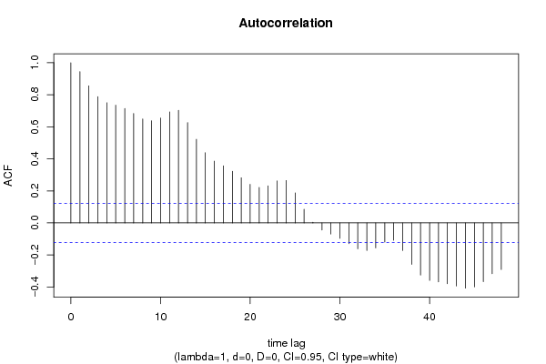
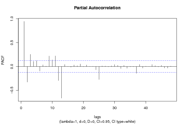
Title produced by software

(Partial) Autocorrelation Function

Date of computation

Tue, 06 Dec 2011 04:05:34 -0500

Cite this page as follows

Statistical Computations at FreeStatistics.org, Office for Research Development and Education, URL https://freestatistics.org/blog/index.php?v=date/2011/Dec/06/t1323162371u71znkufmdh5gzs.htm/, Retrieved Mon, 29 Apr 2024 04:53:08 +0000

Statistical Computations at FreeStatistics.org, Office for Research Development and Education, URL https://freestatistics.org/blog/index.php?pk=151393, Retrieved Mon, 29 Apr 2024 04:53:08 +0000

QR Codes:

Paste this QR Code to cite your computation.

Original text written by user:

IsPrivate?

No (this computation is public)

User-defined keywords

Estimated Impact

126

Family? (F = Feedback message, R = changed R code, M = changed R Module, P = changed Parameters, D = changed Data)

-     [Univariate Data Series] [data set] [2008-12-01 19:54:57] [b98453cac15ba1066b407e146608df68]
- RMP   [(Partial) Autocorrelation Function] [Unemployment] [2010-11-29 09:05:21] [b98453cac15ba1066b407e146608df68]
- R P     [(Partial) Autocorrelation Function] [ws9] [2011-12-04 18:35:07] [8501ca4b76170905b8a207a77f626994]
-    D        [(Partial) Autocorrelation Function] [Workshop 9_Graph1] [2011-12-06 09:05:34] [3e64eea457df40fcb7af8f28e1ee6256] [Current]
- R P           [(Partial) Autocorrelation Function] [Workshop 9_Graph1] [2011-12-06 09:13:56] [f722e8e78b9e5c5ebaa2263f273aa636] 
- RMP             [Standard Deviation-Mean Plot] [Workshop 9_Graph4] [2011-12-06 10:26:02] [f722e8e78b9e5c5ebaa2263f273aa636] 
- RMP           [Spectral Analysis] [Workshop 9_Graph2] [2011-12-06 09:28:52] [f722e8e78b9e5c5ebaa2263f273aa636] 
- R P             [Spectral Analysis] [Workshop 9_Graph2B] [2011-12-06 09:34:36] [f722e8e78b9e5c5ebaa2263f273aa636] 
- R P             [Spectral Analysis] [Workshop 9_Graph2] [2011-12-06 09:35:47] [f722e8e78b9e5c5ebaa2263f273aa636] 
-   PD              [Spectral Analysis] [Paper: CP ] [2011-12-23 11:41:11] [f722e8e78b9e5c5ebaa2263f273aa636] 
-                     [Spectral Analysis] [Paper: Cumulatiev...] [2011-12-23 11:44:50] [f722e8e78b9e5c5ebaa2263f273aa636] 
- RM                  [Variance Reduction Matrix] [Paper: Variance R...] [2011-12-23 11:50:48] [f722e8e78b9e5c5ebaa2263f273aa636] 
- RM                  [Variance Reduction Matrix] [Paper: Variance R...] [2011-12-23 11:50:48] [f722e8e78b9e5c5ebaa2263f273aa636] 
- RM                  [Standard Deviation-Mean Plot] [Paper: Standard D...] [2011-12-23 11:59:05] [f722e8e78b9e5c5ebaa2263f273aa636] 

Feedback Forum

Post a new message

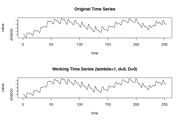
Dataseries X:

Download CSV

Histogram

Boxplots

Summary of computational transaction
Raw Input	view raw input (R code)
Raw Output	view raw output of R engine
Computing time	1 seconds
R Server	'Gwilym Jenkins' @ jenkins.wessa.net

\begin{tabular}{lllllllll}
\hline
Summary of computational transaction \tabularnewline
Raw Input & view raw input (R code)  \tabularnewline
Raw Output & view raw output of R engine  \tabularnewline
Computing time & 1 seconds \tabularnewline
R Server & 'Gwilym Jenkins' @ jenkins.wessa.net \tabularnewline
\hline
\end{tabular}
%Source: https://freestatistics.org/blog/index.php?pk=151393&T=0

[TABLE]
[ROW][C]Summary of computational transaction[/C][/ROW]
[ROW][C]Raw Input[/C][C]view raw input (R code) [/C][/ROW]
[ROW][C]Raw Output[/C][C]view raw output of R engine [/C][/ROW]
[ROW][C]Computing time[/C][C]1 seconds[/C][/ROW]
[ROW][C]R Server[/C][C]'Gwilym Jenkins' @ jenkins.wessa.net[/C][/ROW]
[/TABLE]
Source: https://freestatistics.org/blog/index.php?pk=151393&T=0

Globally Unique Identifier (entire table): ba.freestatistics.org/blog/index.php?pk=151393&T=0

As an alternative you can also use a QR Code:

The GUIDs for individual cells are displayed in the table below:

Summary of computational transaction
Raw Input	view raw input (R code)
Raw Output	view raw output of R engine
Computing time	1 seconds
R Server	'Gwilym Jenkins' @ jenkins.wessa.net

Autocorrelation Function
Time lag k	ACF(k)	T-STAT	P-value
1	0.943952	15.0145	0
2	0.855584	13.6089	0
3	0.788065	12.5349	0
4	0.750328	11.9347	0
5	0.734919	11.6896	0
6	0.714232	11.3605	0
7	0.683046	10.8645	0
8	0.64927	10.3273	0
9	0.637273	10.1364	0
10	0.65426	10.4066	0
11	0.693005	11.0229	0
12	0.702828	11.1792	0
13	0.626293	9.9618	0
14	0.521919	8.3016	0
15	0.438122	6.9688	0
16	0.385328	6.129	0
17	0.356043	5.6632	0
18	0.322737	5.1334	0
19	0.28166	4.4801	6e-06
20	0.240854	3.831	8.1e-05
21	0.221771	3.5275	0.000249
22	0.231492	3.6821	0.000141
23	0.261833	4.1647	2.1e-05
24	0.264646	4.2094	1.8e-05
25	0.187848	2.9879	0.001543
26	0.085373	1.3579	0.087847
27	0.00422	0.0671	0.473267
28	-0.04464	-0.71	0.239168
29	-0.069269	-1.1018	0.135801
30	-0.096291	-1.5316	0.063435
31	-0.129298	-2.0566	0.020375
32	-0.161588	-2.5702	0.005368
33	-0.172236	-2.7396	0.003295
34	-0.155594	-2.4749	0.006992
35	-0.119404	-1.8992	0.029335
36	-0.108444	-1.7249	0.042883
37	-0.171995	-2.7358	0.003332
38	-0.258603	-4.1133	2.6e-05
39	-0.325018	-5.1697	0
40	-0.35902	-5.7106	0
41	-0.368553	-5.8622	0
42	-0.378991	-6.0282	0
43	-0.393934	-6.2659	0
44	-0.407225	-6.4773	0
45	-0.399286	-6.351	0
46	-0.366384	-5.8277	0
47	-0.316471	-5.0338	0
48	-0.290857	-4.6264	3e-06

\begin{tabular}{lllllllll}
\hline
Autocorrelation Function \tabularnewline
Time lag k & ACF(k) & T-STAT & P-value \tabularnewline
1 & 0.943952 & 15.0145 & 0 \tabularnewline
2 & 0.855584 & 13.6089 & 0 \tabularnewline
3 & 0.788065 & 12.5349 & 0 \tabularnewline
4 & 0.750328 & 11.9347 & 0 \tabularnewline
5 & 0.734919 & 11.6896 & 0 \tabularnewline
6 & 0.714232 & 11.3605 & 0 \tabularnewline
7 & 0.683046 & 10.8645 & 0 \tabularnewline
8 & 0.64927 & 10.3273 & 0 \tabularnewline
9 & 0.637273 & 10.1364 & 0 \tabularnewline
10 & 0.65426 & 10.4066 & 0 \tabularnewline
11 & 0.693005 & 11.0229 & 0 \tabularnewline
12 & 0.702828 & 11.1792 & 0 \tabularnewline
13 & 0.626293 & 9.9618 & 0 \tabularnewline
14 & 0.521919 & 8.3016 & 0 \tabularnewline
15 & 0.438122 & 6.9688 & 0 \tabularnewline
16 & 0.385328 & 6.129 & 0 \tabularnewline
17 & 0.356043 & 5.6632 & 0 \tabularnewline
18 & 0.322737 & 5.1334 & 0 \tabularnewline
19 & 0.28166 & 4.4801 & 6e-06 \tabularnewline
20 & 0.240854 & 3.831 & 8.1e-05 \tabularnewline
21 & 0.221771 & 3.5275 & 0.000249 \tabularnewline
22 & 0.231492 & 3.6821 & 0.000141 \tabularnewline
23 & 0.261833 & 4.1647 & 2.1e-05 \tabularnewline
24 & 0.264646 & 4.2094 & 1.8e-05 \tabularnewline
25 & 0.187848 & 2.9879 & 0.001543 \tabularnewline
26 & 0.085373 & 1.3579 & 0.087847 \tabularnewline
27 & 0.00422 & 0.0671 & 0.473267 \tabularnewline
28 & -0.04464 & -0.71 & 0.239168 \tabularnewline
29 & -0.069269 & -1.1018 & 0.135801 \tabularnewline
30 & -0.096291 & -1.5316 & 0.063435 \tabularnewline
31 & -0.129298 & -2.0566 & 0.020375 \tabularnewline
32 & -0.161588 & -2.5702 & 0.005368 \tabularnewline
33 & -0.172236 & -2.7396 & 0.003295 \tabularnewline
34 & -0.155594 & -2.4749 & 0.006992 \tabularnewline
35 & -0.119404 & -1.8992 & 0.029335 \tabularnewline
36 & -0.108444 & -1.7249 & 0.042883 \tabularnewline
37 & -0.171995 & -2.7358 & 0.003332 \tabularnewline
38 & -0.258603 & -4.1133 & 2.6e-05 \tabularnewline
39 & -0.325018 & -5.1697 & 0 \tabularnewline
40 & -0.35902 & -5.7106 & 0 \tabularnewline
41 & -0.368553 & -5.8622 & 0 \tabularnewline
42 & -0.378991 & -6.0282 & 0 \tabularnewline
43 & -0.393934 & -6.2659 & 0 \tabularnewline
44 & -0.407225 & -6.4773 & 0 \tabularnewline
45 & -0.399286 & -6.351 & 0 \tabularnewline
46 & -0.366384 & -5.8277 & 0 \tabularnewline
47 & -0.316471 & -5.0338 & 0 \tabularnewline
48 & -0.290857 & -4.6264 & 3e-06 \tabularnewline
\hline
\end{tabular}
%Source: https://freestatistics.org/blog/index.php?pk=151393&T=1

[TABLE]
[ROW][C]Autocorrelation Function[/C][/ROW]
[ROW][C]Time lag k[/C][C]ACF(k)[/C][C]T-STAT[/C][C]P-value[/C][/ROW]
[ROW][C]1[/C][C]0.943952[/C][C]15.0145[/C][C]0[/C][/ROW]
[ROW][C]2[/C][C]0.855584[/C][C]13.6089[/C][C]0[/C][/ROW]
[ROW][C]3[/C][C]0.788065[/C][C]12.5349[/C][C]0[/C][/ROW]
[ROW][C]4[/C][C]0.750328[/C][C]11.9347[/C][C]0[/C][/ROW]
[ROW][C]5[/C][C]0.734919[/C][C]11.6896[/C][C]0[/C][/ROW]
[ROW][C]6[/C][C]0.714232[/C][C]11.3605[/C][C]0[/C][/ROW]
[ROW][C]7[/C][C]0.683046[/C][C]10.8645[/C][C]0[/C][/ROW]
[ROW][C]8[/C][C]0.64927[/C][C]10.3273[/C][C]0[/C][/ROW]
[ROW][C]9[/C][C]0.637273[/C][C]10.1364[/C][C]0[/C][/ROW]
[ROW][C]10[/C][C]0.65426[/C][C]10.4066[/C][C]0[/C][/ROW]
[ROW][C]11[/C][C]0.693005[/C][C]11.0229[/C][C]0[/C][/ROW]
[ROW][C]12[/C][C]0.702828[/C][C]11.1792[/C][C]0[/C][/ROW]
[ROW][C]13[/C][C]0.626293[/C][C]9.9618[/C][C]0[/C][/ROW]
[ROW][C]14[/C][C]0.521919[/C][C]8.3016[/C][C]0[/C][/ROW]
[ROW][C]15[/C][C]0.438122[/C][C]6.9688[/C][C]0[/C][/ROW]
[ROW][C]16[/C][C]0.385328[/C][C]6.129[/C][C]0[/C][/ROW]
[ROW][C]17[/C][C]0.356043[/C][C]5.6632[/C][C]0[/C][/ROW]
[ROW][C]18[/C][C]0.322737[/C][C]5.1334[/C][C]0[/C][/ROW]
[ROW][C]19[/C][C]0.28166[/C][C]4.4801[/C][C]6e-06[/C][/ROW]
[ROW][C]20[/C][C]0.240854[/C][C]3.831[/C][C]8.1e-05[/C][/ROW]
[ROW][C]21[/C][C]0.221771[/C][C]3.5275[/C][C]0.000249[/C][/ROW]
[ROW][C]22[/C][C]0.231492[/C][C]3.6821[/C][C]0.000141[/C][/ROW]
[ROW][C]23[/C][C]0.261833[/C][C]4.1647[/C][C]2.1e-05[/C][/ROW]
[ROW][C]24[/C][C]0.264646[/C][C]4.2094[/C][C]1.8e-05[/C][/ROW]
[ROW][C]25[/C][C]0.187848[/C][C]2.9879[/C][C]0.001543[/C][/ROW]
[ROW][C]26[/C][C]0.085373[/C][C]1.3579[/C][C]0.087847[/C][/ROW]
[ROW][C]27[/C][C]0.00422[/C][C]0.0671[/C][C]0.473267[/C][/ROW]
[ROW][C]28[/C][C]-0.04464[/C][C]-0.71[/C][C]0.239168[/C][/ROW]
[ROW][C]29[/C][C]-0.069269[/C][C]-1.1018[/C][C]0.135801[/C][/ROW]
[ROW][C]30[/C][C]-0.096291[/C][C]-1.5316[/C][C]0.063435[/C][/ROW]
[ROW][C]31[/C][C]-0.129298[/C][C]-2.0566[/C][C]0.020375[/C][/ROW]
[ROW][C]32[/C][C]-0.161588[/C][C]-2.5702[/C][C]0.005368[/C][/ROW]
[ROW][C]33[/C][C]-0.172236[/C][C]-2.7396[/C][C]0.003295[/C][/ROW]
[ROW][C]34[/C][C]-0.155594[/C][C]-2.4749[/C][C]0.006992[/C][/ROW]
[ROW][C]35[/C][C]-0.119404[/C][C]-1.8992[/C][C]0.029335[/C][/ROW]
[ROW][C]36[/C][C]-0.108444[/C][C]-1.7249[/C][C]0.042883[/C][/ROW]
[ROW][C]37[/C][C]-0.171995[/C][C]-2.7358[/C][C]0.003332[/C][/ROW]
[ROW][C]38[/C][C]-0.258603[/C][C]-4.1133[/C][C]2.6e-05[/C][/ROW]
[ROW][C]39[/C][C]-0.325018[/C][C]-5.1697[/C][C]0[/C][/ROW]
[ROW][C]40[/C][C]-0.35902[/C][C]-5.7106[/C][C]0[/C][/ROW]
[ROW][C]41[/C][C]-0.368553[/C][C]-5.8622[/C][C]0[/C][/ROW]
[ROW][C]42[/C][C]-0.378991[/C][C]-6.0282[/C][C]0[/C][/ROW]
[ROW][C]43[/C][C]-0.393934[/C][C]-6.2659[/C][C]0[/C][/ROW]
[ROW][C]44[/C][C]-0.407225[/C][C]-6.4773[/C][C]0[/C][/ROW]
[ROW][C]45[/C][C]-0.399286[/C][C]-6.351[/C][C]0[/C][/ROW]
[ROW][C]46[/C][C]-0.366384[/C][C]-5.8277[/C][C]0[/C][/ROW]
[ROW][C]47[/C][C]-0.316471[/C][C]-5.0338[/C][C]0[/C][/ROW]
[ROW][C]48[/C][C]-0.290857[/C][C]-4.6264[/C][C]3e-06[/C][/ROW]
[/TABLE]
Source: https://freestatistics.org/blog/index.php?pk=151393&T=1

Globally Unique Identifier (entire table): ba.freestatistics.org/blog/index.php?pk=151393&T=1

As an alternative you can also use a QR Code:

The GUIDs for individual cells are displayed in the table below:

Autocorrelation Function
Time lag k	ACF(k)	T-STAT	P-value
1	0.943952	15.0145	0
2	0.855584	13.6089	0
3	0.788065	12.5349	0
4	0.750328	11.9347	0
5	0.734919	11.6896	0
6	0.714232	11.3605	0
7	0.683046	10.8645	0
8	0.64927	10.3273	0
9	0.637273	10.1364	0
10	0.65426	10.4066	0
11	0.693005	11.0229	0
12	0.702828	11.1792	0
13	0.626293	9.9618	0
14	0.521919	8.3016	0
15	0.438122	6.9688	0
16	0.385328	6.129	0
17	0.356043	5.6632	0
18	0.322737	5.1334	0
19	0.28166	4.4801	6e-06
20	0.240854	3.831	8.1e-05
21	0.221771	3.5275	0.000249
22	0.231492	3.6821	0.000141
23	0.261833	4.1647	2.1e-05
24	0.264646	4.2094	1.8e-05
25	0.187848	2.9879	0.001543
26	0.085373	1.3579	0.087847
27	0.00422	0.0671	0.473267
28	-0.04464	-0.71	0.239168
29	-0.069269	-1.1018	0.135801
30	-0.096291	-1.5316	0.063435
31	-0.129298	-2.0566	0.020375
32	-0.161588	-2.5702	0.005368
33	-0.172236	-2.7396	0.003295
34	-0.155594	-2.4749	0.006992
35	-0.119404	-1.8992	0.029335
36	-0.108444	-1.7249	0.042883
37	-0.171995	-2.7358	0.003332
38	-0.258603	-4.1133	2.6e-05
39	-0.325018	-5.1697	0
40	-0.35902	-5.7106	0
41	-0.368553	-5.8622	0
42	-0.378991	-6.0282	0
43	-0.393934	-6.2659	0
44	-0.407225	-6.4773	0
45	-0.399286	-6.351	0
46	-0.366384	-5.8277	0
47	-0.316471	-5.0338	0
48	-0.290857	-4.6264	3e-06

Partial Autocorrelation Function
Time lag k	PACF(k)	T-STAT	P-value
1	0.943952	15.0145	0
2	-0.325478	-5.177	0
3	0.254631	4.0502	3.4e-05
4	0.106417	1.6927	0.045875
5	0.121826	1.9378	0.026883
6	-0.09558	-1.5203	0.064844
7	0.036317	0.5777	0.282004
8	0.008635	0.1373	0.445432
9	0.219118	3.4853	0.00029
10	0.140026	2.2272	0.013406
11	0.221652	3.5256	0.000251
12	-0.294241	-4.6802	2e-06
13	-0.662101	-10.5314	0
14	0.041945	0.6672	0.252636
15	0.002633	0.0419	0.483316
16	-0.013384	-0.2129	0.415794
17	0.032585	0.5183	0.302351
18	0.016631	0.2645	0.395796
19	0.053203	0.8463	0.199106
20	-0.005091	-0.081	0.467763
21	0.032212	0.5124	0.304419
22	0.001084	0.0172	0.49313
23	0.004066	0.0647	0.474241
24	-0.068491	-1.0894	0.138503
25	-0.272373	-4.3324	1.1e-05
26	0.01269	0.2019	0.420097
27	0.010524	0.1674	0.433596
28	-0.006281	-0.0999	0.460248
29	0.014134	0.2248	0.411151
30	0.040912	0.6507	0.257902
31	0.024284	0.3863	0.349813
32	-0.042297	-0.6728	0.250851
33	0.023143	0.3681	0.356548
34	-0.037256	-0.5926	0.276993
35	-0.006764	-0.1076	0.457206
36	-0.00519	-0.0826	0.467135
37	-0.141611	-2.2525	0.012575
38	0.042126	0.6701	0.251715
39	-0.032929	-0.5238	0.300452
40	0.006097	0.097	0.46141
41	0.002279	0.0362	0.485559
42	0.04246	0.6754	0.25003
43	0.01842	0.293	0.384888
44	-0.008449	-0.1344	0.446598
45	0.02487	0.3956	0.346374
46	-0.031547	-0.5018	0.308128
47	-0.032929	-0.5238	0.300448
48	0.007977	0.1269	0.449566

\begin{tabular}{lllllllll}
\hline
Partial Autocorrelation Function \tabularnewline
Time lag k & PACF(k) & T-STAT & P-value \tabularnewline
1 & 0.943952 & 15.0145 & 0 \tabularnewline
2 & -0.325478 & -5.177 & 0 \tabularnewline
3 & 0.254631 & 4.0502 & 3.4e-05 \tabularnewline
4 & 0.106417 & 1.6927 & 0.045875 \tabularnewline
5 & 0.121826 & 1.9378 & 0.026883 \tabularnewline
6 & -0.09558 & -1.5203 & 0.064844 \tabularnewline
7 & 0.036317 & 0.5777 & 0.282004 \tabularnewline
8 & 0.008635 & 0.1373 & 0.445432 \tabularnewline
9 & 0.219118 & 3.4853 & 0.00029 \tabularnewline
10 & 0.140026 & 2.2272 & 0.013406 \tabularnewline
11 & 0.221652 & 3.5256 & 0.000251 \tabularnewline
12 & -0.294241 & -4.6802 & 2e-06 \tabularnewline
13 & -0.662101 & -10.5314 & 0 \tabularnewline
14 & 0.041945 & 0.6672 & 0.252636 \tabularnewline
15 & 0.002633 & 0.0419 & 0.483316 \tabularnewline
16 & -0.013384 & -0.2129 & 0.415794 \tabularnewline
17 & 0.032585 & 0.5183 & 0.302351 \tabularnewline
18 & 0.016631 & 0.2645 & 0.395796 \tabularnewline
19 & 0.053203 & 0.8463 & 0.199106 \tabularnewline
20 & -0.005091 & -0.081 & 0.467763 \tabularnewline
21 & 0.032212 & 0.5124 & 0.304419 \tabularnewline
22 & 0.001084 & 0.0172 & 0.49313 \tabularnewline
23 & 0.004066 & 0.0647 & 0.474241 \tabularnewline
24 & -0.068491 & -1.0894 & 0.138503 \tabularnewline
25 & -0.272373 & -4.3324 & 1.1e-05 \tabularnewline
26 & 0.01269 & 0.2019 & 0.420097 \tabularnewline
27 & 0.010524 & 0.1674 & 0.433596 \tabularnewline
28 & -0.006281 & -0.0999 & 0.460248 \tabularnewline
29 & 0.014134 & 0.2248 & 0.411151 \tabularnewline
30 & 0.040912 & 0.6507 & 0.257902 \tabularnewline
31 & 0.024284 & 0.3863 & 0.349813 \tabularnewline
32 & -0.042297 & -0.6728 & 0.250851 \tabularnewline
33 & 0.023143 & 0.3681 & 0.356548 \tabularnewline
34 & -0.037256 & -0.5926 & 0.276993 \tabularnewline
35 & -0.006764 & -0.1076 & 0.457206 \tabularnewline
36 & -0.00519 & -0.0826 & 0.467135 \tabularnewline
37 & -0.141611 & -2.2525 & 0.012575 \tabularnewline
38 & 0.042126 & 0.6701 & 0.251715 \tabularnewline
39 & -0.032929 & -0.5238 & 0.300452 \tabularnewline
40 & 0.006097 & 0.097 & 0.46141 \tabularnewline
41 & 0.002279 & 0.0362 & 0.485559 \tabularnewline
42 & 0.04246 & 0.6754 & 0.25003 \tabularnewline
43 & 0.01842 & 0.293 & 0.384888 \tabularnewline
44 & -0.008449 & -0.1344 & 0.446598 \tabularnewline
45 & 0.02487 & 0.3956 & 0.346374 \tabularnewline
46 & -0.031547 & -0.5018 & 0.308128 \tabularnewline
47 & -0.032929 & -0.5238 & 0.300448 \tabularnewline
48 & 0.007977 & 0.1269 & 0.449566 \tabularnewline
\hline
\end{tabular}
%Source: https://freestatistics.org/blog/index.php?pk=151393&T=2

[TABLE]
[ROW][C]Partial Autocorrelation Function[/C][/ROW]
[ROW][C]Time lag k[/C][C]PACF(k)[/C][C]T-STAT[/C][C]P-value[/C][/ROW]
[ROW][C]1[/C][C]0.943952[/C][C]15.0145[/C][C]0[/C][/ROW]
[ROW][C]2[/C][C]-0.325478[/C][C]-5.177[/C][C]0[/C][/ROW]
[ROW][C]3[/C][C]0.254631[/C][C]4.0502[/C][C]3.4e-05[/C][/ROW]
[ROW][C]4[/C][C]0.106417[/C][C]1.6927[/C][C]0.045875[/C][/ROW]
[ROW][C]5[/C][C]0.121826[/C][C]1.9378[/C][C]0.026883[/C][/ROW]
[ROW][C]6[/C][C]-0.09558[/C][C]-1.5203[/C][C]0.064844[/C][/ROW]
[ROW][C]7[/C][C]0.036317[/C][C]0.5777[/C][C]0.282004[/C][/ROW]
[ROW][C]8[/C][C]0.008635[/C][C]0.1373[/C][C]0.445432[/C][/ROW]
[ROW][C]9[/C][C]0.219118[/C][C]3.4853[/C][C]0.00029[/C][/ROW]
[ROW][C]10[/C][C]0.140026[/C][C]2.2272[/C][C]0.013406[/C][/ROW]
[ROW][C]11[/C][C]0.221652[/C][C]3.5256[/C][C]0.000251[/C][/ROW]
[ROW][C]12[/C][C]-0.294241[/C][C]-4.6802[/C][C]2e-06[/C][/ROW]
[ROW][C]13[/C][C]-0.662101[/C][C]-10.5314[/C][C]0[/C][/ROW]
[ROW][C]14[/C][C]0.041945[/C][C]0.6672[/C][C]0.252636[/C][/ROW]
[ROW][C]15[/C][C]0.002633[/C][C]0.0419[/C][C]0.483316[/C][/ROW]
[ROW][C]16[/C][C]-0.013384[/C][C]-0.2129[/C][C]0.415794[/C][/ROW]
[ROW][C]17[/C][C]0.032585[/C][C]0.5183[/C][C]0.302351[/C][/ROW]
[ROW][C]18[/C][C]0.016631[/C][C]0.2645[/C][C]0.395796[/C][/ROW]
[ROW][C]19[/C][C]0.053203[/C][C]0.8463[/C][C]0.199106[/C][/ROW]
[ROW][C]20[/C][C]-0.005091[/C][C]-0.081[/C][C]0.467763[/C][/ROW]
[ROW][C]21[/C][C]0.032212[/C][C]0.5124[/C][C]0.304419[/C][/ROW]
[ROW][C]22[/C][C]0.001084[/C][C]0.0172[/C][C]0.49313[/C][/ROW]
[ROW][C]23[/C][C]0.004066[/C][C]0.0647[/C][C]0.474241[/C][/ROW]
[ROW][C]24[/C][C]-0.068491[/C][C]-1.0894[/C][C]0.138503[/C][/ROW]
[ROW][C]25[/C][C]-0.272373[/C][C]-4.3324[/C][C]1.1e-05[/C][/ROW]
[ROW][C]26[/C][C]0.01269[/C][C]0.2019[/C][C]0.420097[/C][/ROW]
[ROW][C]27[/C][C]0.010524[/C][C]0.1674[/C][C]0.433596[/C][/ROW]
[ROW][C]28[/C][C]-0.006281[/C][C]-0.0999[/C][C]0.460248[/C][/ROW]
[ROW][C]29[/C][C]0.014134[/C][C]0.2248[/C][C]0.411151[/C][/ROW]
[ROW][C]30[/C][C]0.040912[/C][C]0.6507[/C][C]0.257902[/C][/ROW]
[ROW][C]31[/C][C]0.024284[/C][C]0.3863[/C][C]0.349813[/C][/ROW]
[ROW][C]32[/C][C]-0.042297[/C][C]-0.6728[/C][C]0.250851[/C][/ROW]
[ROW][C]33[/C][C]0.023143[/C][C]0.3681[/C][C]0.356548[/C][/ROW]
[ROW][C]34[/C][C]-0.037256[/C][C]-0.5926[/C][C]0.276993[/C][/ROW]
[ROW][C]35[/C][C]-0.006764[/C][C]-0.1076[/C][C]0.457206[/C][/ROW]
[ROW][C]36[/C][C]-0.00519[/C][C]-0.0826[/C][C]0.467135[/C][/ROW]
[ROW][C]37[/C][C]-0.141611[/C][C]-2.2525[/C][C]0.012575[/C][/ROW]
[ROW][C]38[/C][C]0.042126[/C][C]0.6701[/C][C]0.251715[/C][/ROW]
[ROW][C]39[/C][C]-0.032929[/C][C]-0.5238[/C][C]0.300452[/C][/ROW]
[ROW][C]40[/C][C]0.006097[/C][C]0.097[/C][C]0.46141[/C][/ROW]
[ROW][C]41[/C][C]0.002279[/C][C]0.0362[/C][C]0.485559[/C][/ROW]
[ROW][C]42[/C][C]0.04246[/C][C]0.6754[/C][C]0.25003[/C][/ROW]
[ROW][C]43[/C][C]0.01842[/C][C]0.293[/C][C]0.384888[/C][/ROW]
[ROW][C]44[/C][C]-0.008449[/C][C]-0.1344[/C][C]0.446598[/C][/ROW]
[ROW][C]45[/C][C]0.02487[/C][C]0.3956[/C][C]0.346374[/C][/ROW]
[ROW][C]46[/C][C]-0.031547[/C][C]-0.5018[/C][C]0.308128[/C][/ROW]
[ROW][C]47[/C][C]-0.032929[/C][C]-0.5238[/C][C]0.300448[/C][/ROW]
[ROW][C]48[/C][C]0.007977[/C][C]0.1269[/C][C]0.449566[/C][/ROW]
[/TABLE]
Source: https://freestatistics.org/blog/index.php?pk=151393&T=2

Globally Unique Identifier (entire table): ba.freestatistics.org/blog/index.php?pk=151393&T=2

As an alternative you can also use a QR Code:

The GUIDs for individual cells are displayed in the table below:

Partial Autocorrelation Function
Time lag k	PACF(k)	T-STAT	P-value
1	0.943952	15.0145	0
2	-0.325478	-5.177	0
3	0.254631	4.0502	3.4e-05
4	0.106417	1.6927	0.045875
5	0.121826	1.9378	0.026883
6	-0.09558	-1.5203	0.064844
7	0.036317	0.5777	0.282004
8	0.008635	0.1373	0.445432
9	0.219118	3.4853	0.00029
10	0.140026	2.2272	0.013406
11	0.221652	3.5256	0.000251
12	-0.294241	-4.6802	2e-06
13	-0.662101	-10.5314	0
14	0.041945	0.6672	0.252636
15	0.002633	0.0419	0.483316
16	-0.013384	-0.2129	0.415794
17	0.032585	0.5183	0.302351
18	0.016631	0.2645	0.395796
19	0.053203	0.8463	0.199106
20	-0.005091	-0.081	0.467763
21	0.032212	0.5124	0.304419
22	0.001084	0.0172	0.49313
23	0.004066	0.0647	0.474241
24	-0.068491	-1.0894	0.138503
25	-0.272373	-4.3324	1.1e-05
26	0.01269	0.2019	0.420097
27	0.010524	0.1674	0.433596
28	-0.006281	-0.0999	0.460248
29	0.014134	0.2248	0.411151
30	0.040912	0.6507	0.257902
31	0.024284	0.3863	0.349813
32	-0.042297	-0.6728	0.250851
33	0.023143	0.3681	0.356548
34	-0.037256	-0.5926	0.276993
35	-0.006764	-0.1076	0.457206
36	-0.00519	-0.0826	0.467135
37	-0.141611	-2.2525	0.012575
38	0.042126	0.6701	0.251715
39	-0.032929	-0.5238	0.300452
40	0.006097	0.097	0.46141
41	0.002279	0.0362	0.485559
42	0.04246	0.6754	0.25003
43	0.01842	0.293	0.384888
44	-0.008449	-0.1344	0.446598
45	0.02487	0.3956	0.346374
46	-0.031547	-0.5018	0.308128
47	-0.032929	-0.5238	0.300448
48	0.007977	0.1269	0.449566

Figure 1

PNG link

Postscript link

PDF link

Figure 2

PNG link

Postscript link

PDF link

Figure 3

PNG link

Postscript link

PDF link

Parameters (Session):

par1 = 48 ; par2 = 1 ; par3 = 0 ; par4 = 0 ; par5 = 12 ; par6 = White Noise ; par7 = 0.95 ;

Parameters (R input):

par1 = 48 ; par2 = 1 ; par3 = 0 ; par4 = 0 ; par5 = 12 ; par6 = White Noise ; par7 = 0.95 ; par8 = ;

R code (references can be found in the software module):

if (par1 == 'Default') {
par1 = 10*log10(length(x))
} else {
par1 <- as.numeric(par1)
}
par2 <- as.numeric(par2)
par3 <- as.numeric(par3)
par4 <- as.numeric(par4)
par5 <- as.numeric(par5)
if (par6 == 'White Noise') par6 <- 'white' else par6 <- 'ma'
par7 <- as.numeric(par7)
if (par8 != '') par8 <- as.numeric(par8)
ox <- x
if (par8 == '') {
if (par2 == 0) {
x <- log(x)
} else {
x <- (x ^ par2 - 1) / par2
}
} else {
x <- log(x,base=par8)
}
if (par3 > 0) x <- diff(x,lag=1,difference=par3)
if (par4 > 0) x <- diff(x,lag=par5,difference=par4)
bitmap(file='picts.png')
op <- par(mfrow=c(2,1))
plot(ox,type='l',main='Original Time Series',xlab='time',ylab='value')
if (par8=='') {
mytitle <- paste('Working Time Series (lambda=',par2,', d=',par3,', D=',par4,')',sep='')
mysub <- paste('(lambda=',par2,', d=',par3,', D=',par4,', CI=', par7, ', CI type=',par6,')',sep='')
} else {
mytitle <- paste('Working Time Series (base=',par8,', d=',par3,', D=',par4,')',sep='')
mysub <- paste('(base=',par8,', d=',par3,', D=',par4,', CI=', par7, ', CI type=',par6,')',sep='')
}
plot(x,type='l', main=mytitle,xlab='time',ylab='value')
par(op)
dev.off()
bitmap(file='pic1.png')
racf <- acf(x, par1, main='Autocorrelation', xlab='time lag', ylab='ACF', ci.type=par6, ci=par7, sub=mysub)
dev.off()
bitmap(file='pic2.png')
rpacf <- pacf(x,par1,main='Partial Autocorrelation',xlab='lags',ylab='PACF',sub=mysub)
dev.off()
(myacf <- c(racf$acf))
(mypacf <- c(rpacf$acf))
lengthx <- length(x)
sqrtn <- sqrt(lengthx)
load(file='createtable')
a<-table.start()
a<-table.row.start(a)
a<-table.element(a,'Autocorrelation Function',4,TRUE)
a<-table.row.end(a)
a<-table.row.start(a)
a<-table.element(a,'Time lag k',header=TRUE)
a<-table.element(a,hyperlink('basics.htm','ACF(k)','click here for more information about the Autocorrelation Function'),header=TRUE)
a<-table.element(a,'T-STAT',header=TRUE)
a<-table.element(a,'P-value',header=TRUE)
a<-table.row.end(a)
for (i in 2:(par1+1)) {
a<-table.row.start(a)
a<-table.element(a,i-1,header=TRUE)
a<-table.element(a,round(myacf[i],6))
mytstat <- myacf[i]*sqrtn
a<-table.element(a,round(mytstat,4))
a<-table.element(a,round(1-pt(abs(mytstat),lengthx),6))
a<-table.row.end(a)
}
a<-table.end(a)
table.save(a,file='mytable.tab')
a<-table.start()
a<-table.row.start(a)
a<-table.element(a,'Partial Autocorrelation Function',4,TRUE)
a<-table.row.end(a)
a<-table.row.start(a)
a<-table.element(a,'Time lag k',header=TRUE)
a<-table.element(a,hyperlink('basics.htm','PACF(k)','click here for more information about the Partial Autocorrelation Function'),header=TRUE)
a<-table.element(a,'T-STAT',header=TRUE)
a<-table.element(a,'P-value',header=TRUE)
a<-table.row.end(a)
for (i in 1:par1) {
a<-table.row.start(a)
a<-table.element(a,i,header=TRUE)
a<-table.element(a,round(mypacf[i],6))
mytstat <- mypacf[i]*sqrtn
a<-table.element(a,round(mytstat,4))
a<-table.element(a,round(1-pt(abs(mytstat),lengthx),6))
a<-table.row.end(a)
}
a<-table.end(a)
table.save(a,file='mytable1.tab')

Free Statistics

Description of Statistical Computation

Tree of Dependent Computations

Dataset

Tables (Output of Computation)

Figures (Output of Computation)

Input Parameters & R Code