Repository of Reproducible Computations

Free Statistics

of Irreproducible Research!

Author's title

Author

*The author of this computation has been verified*

R Software Module

rwasp_autocorrelation.wasp

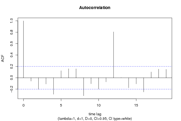
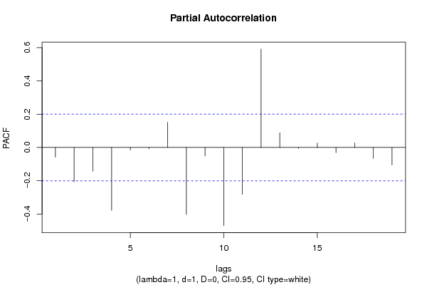
Title produced by software

(Partial) Autocorrelation Function

Date of computation

Tue, 06 Dec 2011 03:08:10 -0500

Cite this page as follows

Statistical Computations at FreeStatistics.org, Office for Research Development and Education, URL https://freestatistics.org/blog/index.php?v=date/2011/Dec/06/t1323158945ngraw3dr4kcx5oh.htm/, Retrieved Sun, 28 Apr 2024 19:25:58 +0000

Statistical Computations at FreeStatistics.org, Office for Research Development and Education, URL https://freestatistics.org/blog/index.php?pk=151371, Retrieved Sun, 28 Apr 2024 19:25:58 +0000

QR Codes:

Paste this QR Code to cite your computation.

Original text written by user:

IsPrivate?

No (this computation is public)

User-defined keywords

Estimated Impact

148

Family? (F = Feedback message, R = changed R code, M = changed R Module, P = changed Parameters, D = changed Data)

-     [Univariate Data Series] [data set] [2008-12-01 19:54:57] [b98453cac15ba1066b407e146608df68]
- RMPD  [(Partial) Autocorrelation Function] [ACF (d=0, D=0)] [2011-12-06 08:00:15] [bcad5ea7a7be31884500e96b7abaff18]
- R P       [(Partial) Autocorrelation Function] [ACF (d=1 en D=0)] [2011-12-06 08:08:10] [d14d64ba86ecc27fb5997ae1bd82937b] [Current]
-   P         [(Partial) Autocorrelation Function] [ACF (d=0, D=1)] [2011-12-06 08:17:43] [bcad5ea7a7be31884500e96b7abaff18] 
-   P           [(Partial) Autocorrelation Function] [ACF (d=1, D=1)] [2011-12-06 08:18:59] [bcad5ea7a7be31884500e96b7abaff18] 
- RMP             [Spectral Analysis] [CP (d=0, D=0)] [2011-12-06 08:24:51] [bcad5ea7a7be31884500e96b7abaff18] 
- R P               [Spectral Analysis] [CP (d=1, D=0)] [2011-12-06 08:27:06] [bcad5ea7a7be31884500e96b7abaff18] 
-   P                 [Spectral Analysis] [CP (d=0, D=1)] [2011-12-06 08:28:42] [bcad5ea7a7be31884500e96b7abaff18] 
-   P                   [Spectral Analysis] [CP (d=1, D=1)] [2011-12-06 08:30:04] [bcad5ea7a7be31884500e96b7abaff18] 
- RMP                   [Variance Reduction Matrix] [VRM ] [2011-12-06 08:41:26] [bcad5ea7a7be31884500e96b7abaff18] 

Feedback Forum

Post a new message

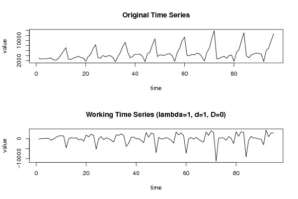
Dataseries X:

Download CSV

Histogram

Boxplots

Summary of computational transaction
Raw Input	view raw input (R code)
Raw Output	view raw output of R engine
Computing time	3 seconds
R Server	'George Udny Yule' @ yule.wessa.net

\begin{tabular}{lllllllll}
\hline
Summary of computational transaction \tabularnewline
Raw Input & view raw input (R code)  \tabularnewline
Raw Output & view raw output of R engine  \tabularnewline
Computing time & 3 seconds \tabularnewline
R Server & 'George Udny Yule' @ yule.wessa.net \tabularnewline
\hline
\end{tabular}
%Source: https://freestatistics.org/blog/index.php?pk=151371&T=0

[TABLE]
[ROW][C]Summary of computational transaction[/C][/ROW]
[ROW][C]Raw Input[/C][C]view raw input (R code) [/C][/ROW]
[ROW][C]Raw Output[/C][C]view raw output of R engine [/C][/ROW]
[ROW][C]Computing time[/C][C]3 seconds[/C][/ROW]
[ROW][C]R Server[/C][C]'George Udny Yule' @ yule.wessa.net[/C][/ROW]
[/TABLE]
Source: https://freestatistics.org/blog/index.php?pk=151371&T=0

Globally Unique Identifier (entire table): ba.freestatistics.org/blog/index.php?pk=151371&T=0

As an alternative you can also use a QR Code:

The GUIDs for individual cells are displayed in the table below:

Summary of computational transaction
Raw Input	view raw input (R code)
Raw Output	view raw output of R engine
Computing time	3 seconds
R Server	'George Udny Yule' @ yule.wessa.net

Autocorrelation Function
Time lag k	ACF(k)	T-STAT	P-value
1	-0.058734	-0.5725	0.284179
2	-0.202186	-1.9707	0.025837
3	-0.109709	-1.0693	0.14382
4	-0.289873	-2.8253	0.002878
5	0.124261	1.2111	0.114422
6	0.158711	1.5469	0.062604
7	0.157588	1.536	0.063933
8	-0.316618	-3.086	0.001329
9	-0.105371	-1.027	0.153507
10	-0.197365	-1.9237	0.028695
11	-0.072642	-0.708	0.240332
12	0.806601	7.8618	0
13	0.003435	0.0335	0.48668
14	-0.176082	-1.7162	0.044689
15	-0.107184	-1.0447	0.149406
16	-0.249232	-2.4292	0.008506
17	0.102081	0.995	0.161142
18	0.151355	1.4752	0.071729
19	0.148398	1.4464	0.075677

\begin{tabular}{lllllllll}
\hline
Autocorrelation Function \tabularnewline
Time lag k & ACF(k) & T-STAT & P-value \tabularnewline
1 & -0.058734 & -0.5725 & 0.284179 \tabularnewline
2 & -0.202186 & -1.9707 & 0.025837 \tabularnewline
3 & -0.109709 & -1.0693 & 0.14382 \tabularnewline
4 & -0.289873 & -2.8253 & 0.002878 \tabularnewline
5 & 0.124261 & 1.2111 & 0.114422 \tabularnewline
6 & 0.158711 & 1.5469 & 0.062604 \tabularnewline
7 & 0.157588 & 1.536 & 0.063933 \tabularnewline
8 & -0.316618 & -3.086 & 0.001329 \tabularnewline
9 & -0.105371 & -1.027 & 0.153507 \tabularnewline
10 & -0.197365 & -1.9237 & 0.028695 \tabularnewline
11 & -0.072642 & -0.708 & 0.240332 \tabularnewline
12 & 0.806601 & 7.8618 & 0 \tabularnewline
13 & 0.003435 & 0.0335 & 0.48668 \tabularnewline
14 & -0.176082 & -1.7162 & 0.044689 \tabularnewline
15 & -0.107184 & -1.0447 & 0.149406 \tabularnewline
16 & -0.249232 & -2.4292 & 0.008506 \tabularnewline
17 & 0.102081 & 0.995 & 0.161142 \tabularnewline
18 & 0.151355 & 1.4752 & 0.071729 \tabularnewline
19 & 0.148398 & 1.4464 & 0.075677 \tabularnewline
\hline
\end{tabular}
%Source: https://freestatistics.org/blog/index.php?pk=151371&T=1

[TABLE]
[ROW][C]Autocorrelation Function[/C][/ROW]
[ROW][C]Time lag k[/C][C]ACF(k)[/C][C]T-STAT[/C][C]P-value[/C][/ROW]
[ROW][C]1[/C][C]-0.058734[/C][C]-0.5725[/C][C]0.284179[/C][/ROW]
[ROW][C]2[/C][C]-0.202186[/C][C]-1.9707[/C][C]0.025837[/C][/ROW]
[ROW][C]3[/C][C]-0.109709[/C][C]-1.0693[/C][C]0.14382[/C][/ROW]
[ROW][C]4[/C][C]-0.289873[/C][C]-2.8253[/C][C]0.002878[/C][/ROW]
[ROW][C]5[/C][C]0.124261[/C][C]1.2111[/C][C]0.114422[/C][/ROW]
[ROW][C]6[/C][C]0.158711[/C][C]1.5469[/C][C]0.062604[/C][/ROW]
[ROW][C]7[/C][C]0.157588[/C][C]1.536[/C][C]0.063933[/C][/ROW]
[ROW][C]8[/C][C]-0.316618[/C][C]-3.086[/C][C]0.001329[/C][/ROW]
[ROW][C]9[/C][C]-0.105371[/C][C]-1.027[/C][C]0.153507[/C][/ROW]
[ROW][C]10[/C][C]-0.197365[/C][C]-1.9237[/C][C]0.028695[/C][/ROW]
[ROW][C]11[/C][C]-0.072642[/C][C]-0.708[/C][C]0.240332[/C][/ROW]
[ROW][C]12[/C][C]0.806601[/C][C]7.8618[/C][C]0[/C][/ROW]
[ROW][C]13[/C][C]0.003435[/C][C]0.0335[/C][C]0.48668[/C][/ROW]
[ROW][C]14[/C][C]-0.176082[/C][C]-1.7162[/C][C]0.044689[/C][/ROW]
[ROW][C]15[/C][C]-0.107184[/C][C]-1.0447[/C][C]0.149406[/C][/ROW]
[ROW][C]16[/C][C]-0.249232[/C][C]-2.4292[/C][C]0.008506[/C][/ROW]
[ROW][C]17[/C][C]0.102081[/C][C]0.995[/C][C]0.161142[/C][/ROW]
[ROW][C]18[/C][C]0.151355[/C][C]1.4752[/C][C]0.071729[/C][/ROW]
[ROW][C]19[/C][C]0.148398[/C][C]1.4464[/C][C]0.075677[/C][/ROW]
[/TABLE]
Source: https://freestatistics.org/blog/index.php?pk=151371&T=1

Globally Unique Identifier (entire table): ba.freestatistics.org/blog/index.php?pk=151371&T=1

As an alternative you can also use a QR Code:

The GUIDs for individual cells are displayed in the table below:

Autocorrelation Function
Time lag k	ACF(k)	T-STAT	P-value
1	-0.058734	-0.5725	0.284179
2	-0.202186	-1.9707	0.025837
3	-0.109709	-1.0693	0.14382
4	-0.289873	-2.8253	0.002878
5	0.124261	1.2111	0.114422
6	0.158711	1.5469	0.062604
7	0.157588	1.536	0.063933
8	-0.316618	-3.086	0.001329
9	-0.105371	-1.027	0.153507
10	-0.197365	-1.9237	0.028695
11	-0.072642	-0.708	0.240332
12	0.806601	7.8618	0
13	0.003435	0.0335	0.48668
14	-0.176082	-1.7162	0.044689
15	-0.107184	-1.0447	0.149406
16	-0.249232	-2.4292	0.008506
17	0.102081	0.995	0.161142
18	0.151355	1.4752	0.071729
19	0.148398	1.4464	0.075677

Partial Autocorrelation Function
Time lag k	PACF(k)	T-STAT	P-value
1	-0.058734	-0.5725	0.284179
2	-0.206347	-2.0112	0.023568
3	-0.142701	-1.3909	0.083756
4	-0.37769	-3.6813	0.000193
5	-0.014784	-0.1441	0.442863
6	-0.008288	-0.0808	0.467892
7	0.151005	1.4718	0.072188
8	-0.402506	-3.9231	8.3e-05
9	-0.051129	-0.4983	0.309696
10	-0.470005	-4.581	7e-06
11	-0.281395	-2.7427	0.003642
12	0.591391	5.7642	0
13	0.089021	0.8677	0.19388
14	-0.00521	-0.0508	0.479805
15	0.026269	0.256	0.399238
16	-0.03101	-0.3022	0.381562
17	0.028088	0.2738	0.392427
18	-0.065391	-0.6374	0.262713
19	-0.104737	-1.0208	0.15496

\begin{tabular}{lllllllll}
\hline
Partial Autocorrelation Function \tabularnewline
Time lag k & PACF(k) & T-STAT & P-value \tabularnewline
1 & -0.058734 & -0.5725 & 0.284179 \tabularnewline
2 & -0.206347 & -2.0112 & 0.023568 \tabularnewline
3 & -0.142701 & -1.3909 & 0.083756 \tabularnewline
4 & -0.37769 & -3.6813 & 0.000193 \tabularnewline
5 & -0.014784 & -0.1441 & 0.442863 \tabularnewline
6 & -0.008288 & -0.0808 & 0.467892 \tabularnewline
7 & 0.151005 & 1.4718 & 0.072188 \tabularnewline
8 & -0.402506 & -3.9231 & 8.3e-05 \tabularnewline
9 & -0.051129 & -0.4983 & 0.309696 \tabularnewline
10 & -0.470005 & -4.581 & 7e-06 \tabularnewline
11 & -0.281395 & -2.7427 & 0.003642 \tabularnewline
12 & 0.591391 & 5.7642 & 0 \tabularnewline
13 & 0.089021 & 0.8677 & 0.19388 \tabularnewline
14 & -0.00521 & -0.0508 & 0.479805 \tabularnewline
15 & 0.026269 & 0.256 & 0.399238 \tabularnewline
16 & -0.03101 & -0.3022 & 0.381562 \tabularnewline
17 & 0.028088 & 0.2738 & 0.392427 \tabularnewline
18 & -0.065391 & -0.6374 & 0.262713 \tabularnewline
19 & -0.104737 & -1.0208 & 0.15496 \tabularnewline
\hline
\end{tabular}
%Source: https://freestatistics.org/blog/index.php?pk=151371&T=2

[TABLE]
[ROW][C]Partial Autocorrelation Function[/C][/ROW]
[ROW][C]Time lag k[/C][C]PACF(k)[/C][C]T-STAT[/C][C]P-value[/C][/ROW]
[ROW][C]1[/C][C]-0.058734[/C][C]-0.5725[/C][C]0.284179[/C][/ROW]
[ROW][C]2[/C][C]-0.206347[/C][C]-2.0112[/C][C]0.023568[/C][/ROW]
[ROW][C]3[/C][C]-0.142701[/C][C]-1.3909[/C][C]0.083756[/C][/ROW]
[ROW][C]4[/C][C]-0.37769[/C][C]-3.6813[/C][C]0.000193[/C][/ROW]
[ROW][C]5[/C][C]-0.014784[/C][C]-0.1441[/C][C]0.442863[/C][/ROW]
[ROW][C]6[/C][C]-0.008288[/C][C]-0.0808[/C][C]0.467892[/C][/ROW]
[ROW][C]7[/C][C]0.151005[/C][C]1.4718[/C][C]0.072188[/C][/ROW]
[ROW][C]8[/C][C]-0.402506[/C][C]-3.9231[/C][C]8.3e-05[/C][/ROW]
[ROW][C]9[/C][C]-0.051129[/C][C]-0.4983[/C][C]0.309696[/C][/ROW]
[ROW][C]10[/C][C]-0.470005[/C][C]-4.581[/C][C]7e-06[/C][/ROW]
[ROW][C]11[/C][C]-0.281395[/C][C]-2.7427[/C][C]0.003642[/C][/ROW]
[ROW][C]12[/C][C]0.591391[/C][C]5.7642[/C][C]0[/C][/ROW]
[ROW][C]13[/C][C]0.089021[/C][C]0.8677[/C][C]0.19388[/C][/ROW]
[ROW][C]14[/C][C]-0.00521[/C][C]-0.0508[/C][C]0.479805[/C][/ROW]
[ROW][C]15[/C][C]0.026269[/C][C]0.256[/C][C]0.399238[/C][/ROW]
[ROW][C]16[/C][C]-0.03101[/C][C]-0.3022[/C][C]0.381562[/C][/ROW]
[ROW][C]17[/C][C]0.028088[/C][C]0.2738[/C][C]0.392427[/C][/ROW]
[ROW][C]18[/C][C]-0.065391[/C][C]-0.6374[/C][C]0.262713[/C][/ROW]
[ROW][C]19[/C][C]-0.104737[/C][C]-1.0208[/C][C]0.15496[/C][/ROW]
[/TABLE]
Source: https://freestatistics.org/blog/index.php?pk=151371&T=2

Globally Unique Identifier (entire table): ba.freestatistics.org/blog/index.php?pk=151371&T=2

As an alternative you can also use a QR Code:

The GUIDs for individual cells are displayed in the table below:

Partial Autocorrelation Function
Time lag k	PACF(k)	T-STAT	P-value
1	-0.058734	-0.5725	0.284179
2	-0.206347	-2.0112	0.023568
3	-0.142701	-1.3909	0.083756
4	-0.37769	-3.6813	0.000193
5	-0.014784	-0.1441	0.442863
6	-0.008288	-0.0808	0.467892
7	0.151005	1.4718	0.072188
8	-0.402506	-3.9231	8.3e-05
9	-0.051129	-0.4983	0.309696
10	-0.470005	-4.581	7e-06
11	-0.281395	-2.7427	0.003642
12	0.591391	5.7642	0
13	0.089021	0.8677	0.19388
14	-0.00521	-0.0508	0.479805
15	0.026269	0.256	0.399238
16	-0.03101	-0.3022	0.381562
17	0.028088	0.2738	0.392427
18	-0.065391	-0.6374	0.262713
19	-0.104737	-1.0208	0.15496

Figure 1

PNG link

Postscript link

PDF link

Figure 2

PNG link

Postscript link

PDF link

Figure 3

PNG link

Postscript link

PDF link

Parameters (Session):

par1 = Default ; par2 = 1 ; par3 = 1 ; par4 = 0 ; par5 = 12 ; par6 = White Noise ; par7 = 0.95 ;

Parameters (R input):

par1 = Default ; par2 = 1 ; par3 = 1 ; par4 = 0 ; par5 = 12 ; par6 = White Noise ; par7 = 0.95 ; par8 = ;

R code (references can be found in the software module):

if (par1 == 'Default') {
par1 = 10*log10(length(x))
} else {
par1 <- as.numeric(par1)
}
par2 <- as.numeric(par2)
par3 <- as.numeric(par3)
par4 <- as.numeric(par4)
par5 <- as.numeric(par5)
if (par6 == 'White Noise') par6 <- 'white' else par6 <- 'ma'
par7 <- as.numeric(par7)
if (par8 != '') par8 <- as.numeric(par8)
ox <- x
if (par8 == '') {
if (par2 == 0) {
x <- log(x)
} else {
x <- (x ^ par2 - 1) / par2
}
} else {
x <- log(x,base=par8)
}
if (par3 > 0) x <- diff(x,lag=1,difference=par3)
if (par4 > 0) x <- diff(x,lag=par5,difference=par4)
bitmap(file='picts.png')
op <- par(mfrow=c(2,1))
plot(ox,type='l',main='Original Time Series',xlab='time',ylab='value')
if (par8=='') {
mytitle <- paste('Working Time Series (lambda=',par2,', d=',par3,', D=',par4,')',sep='')
mysub <- paste('(lambda=',par2,', d=',par3,', D=',par4,', CI=', par7, ', CI type=',par6,')',sep='')
} else {
mytitle <- paste('Working Time Series (base=',par8,', d=',par3,', D=',par4,')',sep='')
mysub <- paste('(base=',par8,', d=',par3,', D=',par4,', CI=', par7, ', CI type=',par6,')',sep='')
}
plot(x,type='l', main=mytitle,xlab='time',ylab='value')
par(op)
dev.off()
bitmap(file='pic1.png')
racf <- acf(x, par1, main='Autocorrelation', xlab='time lag', ylab='ACF', ci.type=par6, ci=par7, sub=mysub)
dev.off()
bitmap(file='pic2.png')
rpacf <- pacf(x,par1,main='Partial Autocorrelation',xlab='lags',ylab='PACF',sub=mysub)
dev.off()
(myacf <- c(racf$acf))
(mypacf <- c(rpacf$acf))
lengthx <- length(x)
sqrtn <- sqrt(lengthx)
load(file='createtable')
a<-table.start()
a<-table.row.start(a)
a<-table.element(a,'Autocorrelation Function',4,TRUE)
a<-table.row.end(a)
a<-table.row.start(a)
a<-table.element(a,'Time lag k',header=TRUE)
a<-table.element(a,hyperlink('basics.htm','ACF(k)','click here for more information about the Autocorrelation Function'),header=TRUE)
a<-table.element(a,'T-STAT',header=TRUE)
a<-table.element(a,'P-value',header=TRUE)
a<-table.row.end(a)
for (i in 2:(par1+1)) {
a<-table.row.start(a)
a<-table.element(a,i-1,header=TRUE)
a<-table.element(a,round(myacf[i],6))
mytstat <- myacf[i]*sqrtn
a<-table.element(a,round(mytstat,4))
a<-table.element(a,round(1-pt(abs(mytstat),lengthx),6))
a<-table.row.end(a)
}
a<-table.end(a)
table.save(a,file='mytable.tab')
a<-table.start()
a<-table.row.start(a)
a<-table.element(a,'Partial Autocorrelation Function',4,TRUE)
a<-table.row.end(a)
a<-table.row.start(a)
a<-table.element(a,'Time lag k',header=TRUE)
a<-table.element(a,hyperlink('basics.htm','PACF(k)','click here for more information about the Partial Autocorrelation Function'),header=TRUE)
a<-table.element(a,'T-STAT',header=TRUE)
a<-table.element(a,'P-value',header=TRUE)
a<-table.row.end(a)
for (i in 1:par1) {
a<-table.row.start(a)
a<-table.element(a,i,header=TRUE)
a<-table.element(a,round(mypacf[i],6))
mytstat <- mypacf[i]*sqrtn
a<-table.element(a,round(mytstat,4))
a<-table.element(a,round(1-pt(abs(mytstat),lengthx),6))
a<-table.row.end(a)
}
a<-table.end(a)
table.save(a,file='mytable1.tab')

Free Statistics

Description of Statistical Computation

Tree of Dependent Computations

Dataset

Tables (Output of Computation)

Figures (Output of Computation)

Input Parameters & R Code