Repository of Reproducible Computations

Free Statistics

of Irreproducible Research!

Author's title

Author

*The author of this computation has been verified*

R Software Module

rwasp_autocorrelation.wasp

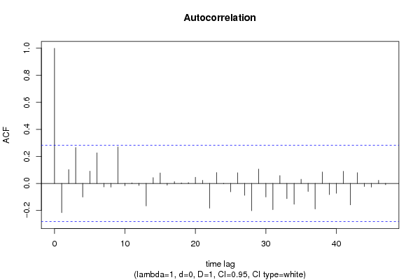
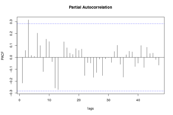
Title produced by software

(Partial) Autocorrelation Function

Date of computation

Mon, 05 Dec 2011 14:35:13 -0500

Cite this page as follows

Statistical Computations at FreeStatistics.org, Office for Research Development and Education, URL https://freestatistics.org/blog/index.php?v=date/2011/Dec/05/t13231137523mg30kdyuv0pif1.htm/, Retrieved Fri, 03 May 2024 14:20:51 +0000

Statistical Computations at FreeStatistics.org, Office for Research Development and Education, URL https://freestatistics.org/blog/index.php?pk=151210, Retrieved Fri, 03 May 2024 14:20:51 +0000

QR Codes:

Paste this QR Code to cite your computation.

Original text written by user:

IsPrivate?

No (this computation is public)

User-defined keywords

Estimated Impact

148

Family? (F = Feedback message, R = changed R code, M = changed R Module, P = changed Parameters, D = changed Data)

-     [Univariate Explorative Data Analysis] [Run Sequence gebo...] [2008-12-12 13:32:37] [76963dc1903f0f612b6153510a3818cf]
- R  D  [Univariate Explorative Data Analysis] [Run Sequence gebo...] [2008-12-17 12:14:40] [76963dc1903f0f612b6153510a3818cf]
-         [Univariate Explorative Data Analysis] [Run Sequence Plot...] [2008-12-22 18:19:51] [1ce0d16c8f4225c977b42c8fa93bc163]
- RMP       [Univariate Data Series] [Identifying Integ...] [2009-11-22 12:08:06] [b98453cac15ba1066b407e146608df68]
- RMP         [(Partial) Autocorrelation Function] [Births] [2010-11-29 09:36:27] [b98453cac15ba1066b407e146608df68]
- R PD          [(Partial) Autocorrelation Function] [WS9 3.1 ACF d=0, D=0] [2010-12-07 10:00:49] [afe9379cca749d06b3d6872e02cc47ed]
- R  D            [(Partial) Autocorrelation Function] [ws9-2] [2011-12-05 18:26:48] [f7a862281046b7153543b12c78921b36]
-   P               [(Partial) Autocorrelation Function] [ws9-3] [2011-12-05 18:35:17] [f7a862281046b7153543b12c78921b36]
-   P                 [(Partial) Autocorrelation Function] [ws9-4] [2011-12-05 18:43:50] [f7a862281046b7153543b12c78921b36]
-   P                   [(Partial) Autocorrelation Function] [ws9-4] [2011-12-05 18:46:25] [f7a862281046b7153543b12c78921b36]
-   P                     [(Partial) Autocorrelation Function] [ws9-4] [2011-12-05 19:34:03] [f7a862281046b7153543b12c78921b36]
-                             [(Partial) Autocorrelation Function] [ws9-4] [2011-12-05 19:35:13] [47995d3a8fac585eeb070a274b466f8c] [Current]
-  MP                           [(Partial) Autocorrelation Function] [paper2-3] [2011-12-21 20:49:59] [f7a862281046b7153543b12c78921b36] 

Feedback Forum

Post a new message

Dataseries X:

Download CSV

Histogram

Boxplots

Summary of computational transaction
Raw Input	view raw input (R code)
Raw Output	view raw output of R engine
Computing time	1 seconds
R Server	'Gertrude Mary Cox' @ cox.wessa.net

\begin{tabular}{lllllllll}
\hline
Summary of computational transaction \tabularnewline
Raw Input & view raw input (R code)  \tabularnewline
Raw Output & view raw output of R engine  \tabularnewline
Computing time & 1 seconds \tabularnewline
R Server & 'Gertrude Mary Cox' @ cox.wessa.net \tabularnewline
\hline
\end{tabular}
%Source: https://freestatistics.org/blog/index.php?pk=151210&T=0

[TABLE]
[ROW][C]Summary of computational transaction[/C][/ROW]
[ROW][C]Raw Input[/C][C]view raw input (R code) [/C][/ROW]
[ROW][C]Raw Output[/C][C]view raw output of R engine [/C][/ROW]
[ROW][C]Computing time[/C][C]1 seconds[/C][/ROW]
[ROW][C]R Server[/C][C]'Gertrude Mary Cox' @ cox.wessa.net[/C][/ROW]
[/TABLE]
Source: https://freestatistics.org/blog/index.php?pk=151210&T=0

Globally Unique Identifier (entire table): ba.freestatistics.org/blog/index.php?pk=151210&T=0

As an alternative you can also use a QR Code:

The GUIDs for individual cells are displayed in the table below:

Summary of computational transaction
Raw Input	view raw input (R code)
Raw Output	view raw output of R engine
Computing time	1 seconds
R Server	'Gertrude Mary Cox' @ cox.wessa.net

Autocorrelation Function
Time lag k	ACF(k)	T-STAT	P-value
1	-0.215962	-1.4962	0.070571
2	0.102587	0.7107	0.240342
3	0.265975	1.8427	0.035774
4	-0.100646	-0.6973	0.244492
5	0.091187	0.6318	0.265271
6	0.226345	1.5682	0.061707
7	-0.025403	-0.176	0.430517
8	-0.027057	-0.1875	0.426047
9	0.270334	1.8729	0.033587
10	-0.01671	-0.1158	0.454159
11	0.004398	0.0305	0.487909
12	-0.015385	-0.1066	0.457778
13	-0.166171	-1.1513	0.127662
14	0.042571	0.2949	0.384655
15	0.077437	0.5365	0.297047
16	-0.012706	-0.088	0.465109
17	0.013255	0.0918	0.463606
18	0.003874	0.0268	0.489349
19	0.005904	0.0409	0.483771
20	0.045443	0.3148	0.377125
21	0.022666	0.157	0.437937
22	-0.183116	-1.2687	0.10534
23	0.080395	0.557	0.29006
24	-0.002976	-0.0206	0.491817
25	-0.062426	-0.4325	0.333658
26	0.078524	0.544	0.294469
27	-0.088356	-0.6121	0.271665
28	-0.201985	-1.3994	0.084062
29	0.106077	0.7349	0.23298
30	-0.100273	-0.6947	0.245293
31	-0.194216	-1.3456	0.092382
32	0.058007	0.4019	0.344776
33	-0.112195	-0.7773	0.220395
34	-0.15375	-1.0652	0.146055
35	0.030562	0.2117	0.416603
36	-0.059281	-0.4107	0.341555
37	-0.188751	-1.3077	0.098602
38	0.084257	0.5838	0.28106
39	-0.083015	-0.5751	0.28394
40	-0.072861	-0.5048	0.308006
41	0.089501	0.6201	0.269069
42	-0.158442	-1.0977	0.138902
43	0.079349	0.5497	0.29252
44	-0.022543	-0.1562	0.438272
45	-0.02749	-0.1905	0.424877
46	0.022775	0.1578	0.437642
47	-0.009709	-0.0673	0.473325
48	NA	NA	NA

\begin{tabular}{lllllllll}
\hline
Autocorrelation Function \tabularnewline
Time lag k & ACF(k) & T-STAT & P-value \tabularnewline
1 & -0.215962 & -1.4962 & 0.070571 \tabularnewline
2 & 0.102587 & 0.7107 & 0.240342 \tabularnewline
3 & 0.265975 & 1.8427 & 0.035774 \tabularnewline
4 & -0.100646 & -0.6973 & 0.244492 \tabularnewline
5 & 0.091187 & 0.6318 & 0.265271 \tabularnewline
6 & 0.226345 & 1.5682 & 0.061707 \tabularnewline
7 & -0.025403 & -0.176 & 0.430517 \tabularnewline
8 & -0.027057 & -0.1875 & 0.426047 \tabularnewline
9 & 0.270334 & 1.8729 & 0.033587 \tabularnewline
10 & -0.01671 & -0.1158 & 0.454159 \tabularnewline
11 & 0.004398 & 0.0305 & 0.487909 \tabularnewline
12 & -0.015385 & -0.1066 & 0.457778 \tabularnewline
13 & -0.166171 & -1.1513 & 0.127662 \tabularnewline
14 & 0.042571 & 0.2949 & 0.384655 \tabularnewline
15 & 0.077437 & 0.5365 & 0.297047 \tabularnewline
16 & -0.012706 & -0.088 & 0.465109 \tabularnewline
17 & 0.013255 & 0.0918 & 0.463606 \tabularnewline
18 & 0.003874 & 0.0268 & 0.489349 \tabularnewline
19 & 0.005904 & 0.0409 & 0.483771 \tabularnewline
20 & 0.045443 & 0.3148 & 0.377125 \tabularnewline
21 & 0.022666 & 0.157 & 0.437937 \tabularnewline
22 & -0.183116 & -1.2687 & 0.10534 \tabularnewline
23 & 0.080395 & 0.557 & 0.29006 \tabularnewline
24 & -0.002976 & -0.0206 & 0.491817 \tabularnewline
25 & -0.062426 & -0.4325 & 0.333658 \tabularnewline
26 & 0.078524 & 0.544 & 0.294469 \tabularnewline
27 & -0.088356 & -0.6121 & 0.271665 \tabularnewline
28 & -0.201985 & -1.3994 & 0.084062 \tabularnewline
29 & 0.106077 & 0.7349 & 0.23298 \tabularnewline
30 & -0.100273 & -0.6947 & 0.245293 \tabularnewline
31 & -0.194216 & -1.3456 & 0.092382 \tabularnewline
32 & 0.058007 & 0.4019 & 0.344776 \tabularnewline
33 & -0.112195 & -0.7773 & 0.220395 \tabularnewline
34 & -0.15375 & -1.0652 & 0.146055 \tabularnewline
35 & 0.030562 & 0.2117 & 0.416603 \tabularnewline
36 & -0.059281 & -0.4107 & 0.341555 \tabularnewline
37 & -0.188751 & -1.3077 & 0.098602 \tabularnewline
38 & 0.084257 & 0.5838 & 0.28106 \tabularnewline
39 & -0.083015 & -0.5751 & 0.28394 \tabularnewline
40 & -0.072861 & -0.5048 & 0.308006 \tabularnewline
41 & 0.089501 & 0.6201 & 0.269069 \tabularnewline
42 & -0.158442 & -1.0977 & 0.138902 \tabularnewline
43 & 0.079349 & 0.5497 & 0.29252 \tabularnewline
44 & -0.022543 & -0.1562 & 0.438272 \tabularnewline
45 & -0.02749 & -0.1905 & 0.424877 \tabularnewline
46 & 0.022775 & 0.1578 & 0.437642 \tabularnewline
47 & -0.009709 & -0.0673 & 0.473325 \tabularnewline
48 & NA & NA & NA \tabularnewline
\hline
\end{tabular}
%Source: https://freestatistics.org/blog/index.php?pk=151210&T=1

[TABLE]
[ROW][C]Autocorrelation Function[/C][/ROW]
[ROW][C]Time lag k[/C][C]ACF(k)[/C][C]T-STAT[/C][C]P-value[/C][/ROW]
[ROW][C]1[/C][C]-0.215962[/C][C]-1.4962[/C][C]0.070571[/C][/ROW]
[ROW][C]2[/C][C]0.102587[/C][C]0.7107[/C][C]0.240342[/C][/ROW]
[ROW][C]3[/C][C]0.265975[/C][C]1.8427[/C][C]0.035774[/C][/ROW]
[ROW][C]4[/C][C]-0.100646[/C][C]-0.6973[/C][C]0.244492[/C][/ROW]
[ROW][C]5[/C][C]0.091187[/C][C]0.6318[/C][C]0.265271[/C][/ROW]
[ROW][C]6[/C][C]0.226345[/C][C]1.5682[/C][C]0.061707[/C][/ROW]
[ROW][C]7[/C][C]-0.025403[/C][C]-0.176[/C][C]0.430517[/C][/ROW]
[ROW][C]8[/C][C]-0.027057[/C][C]-0.1875[/C][C]0.426047[/C][/ROW]
[ROW][C]9[/C][C]0.270334[/C][C]1.8729[/C][C]0.033587[/C][/ROW]
[ROW][C]10[/C][C]-0.01671[/C][C]-0.1158[/C][C]0.454159[/C][/ROW]
[ROW][C]11[/C][C]0.004398[/C][C]0.0305[/C][C]0.487909[/C][/ROW]
[ROW][C]12[/C][C]-0.015385[/C][C]-0.1066[/C][C]0.457778[/C][/ROW]
[ROW][C]13[/C][C]-0.166171[/C][C]-1.1513[/C][C]0.127662[/C][/ROW]
[ROW][C]14[/C][C]0.042571[/C][C]0.2949[/C][C]0.384655[/C][/ROW]
[ROW][C]15[/C][C]0.077437[/C][C]0.5365[/C][C]0.297047[/C][/ROW]
[ROW][C]16[/C][C]-0.012706[/C][C]-0.088[/C][C]0.465109[/C][/ROW]
[ROW][C]17[/C][C]0.013255[/C][C]0.0918[/C][C]0.463606[/C][/ROW]
[ROW][C]18[/C][C]0.003874[/C][C]0.0268[/C][C]0.489349[/C][/ROW]
[ROW][C]19[/C][C]0.005904[/C][C]0.0409[/C][C]0.483771[/C][/ROW]
[ROW][C]20[/C][C]0.045443[/C][C]0.3148[/C][C]0.377125[/C][/ROW]
[ROW][C]21[/C][C]0.022666[/C][C]0.157[/C][C]0.437937[/C][/ROW]
[ROW][C]22[/C][C]-0.183116[/C][C]-1.2687[/C][C]0.10534[/C][/ROW]
[ROW][C]23[/C][C]0.080395[/C][C]0.557[/C][C]0.29006[/C][/ROW]
[ROW][C]24[/C][C]-0.002976[/C][C]-0.0206[/C][C]0.491817[/C][/ROW]
[ROW][C]25[/C][C]-0.062426[/C][C]-0.4325[/C][C]0.333658[/C][/ROW]
[ROW][C]26[/C][C]0.078524[/C][C]0.544[/C][C]0.294469[/C][/ROW]
[ROW][C]27[/C][C]-0.088356[/C][C]-0.6121[/C][C]0.271665[/C][/ROW]
[ROW][C]28[/C][C]-0.201985[/C][C]-1.3994[/C][C]0.084062[/C][/ROW]
[ROW][C]29[/C][C]0.106077[/C][C]0.7349[/C][C]0.23298[/C][/ROW]
[ROW][C]30[/C][C]-0.100273[/C][C]-0.6947[/C][C]0.245293[/C][/ROW]
[ROW][C]31[/C][C]-0.194216[/C][C]-1.3456[/C][C]0.092382[/C][/ROW]
[ROW][C]32[/C][C]0.058007[/C][C]0.4019[/C][C]0.344776[/C][/ROW]
[ROW][C]33[/C][C]-0.112195[/C][C]-0.7773[/C][C]0.220395[/C][/ROW]
[ROW][C]34[/C][C]-0.15375[/C][C]-1.0652[/C][C]0.146055[/C][/ROW]
[ROW][C]35[/C][C]0.030562[/C][C]0.2117[/C][C]0.416603[/C][/ROW]
[ROW][C]36[/C][C]-0.059281[/C][C]-0.4107[/C][C]0.341555[/C][/ROW]
[ROW][C]37[/C][C]-0.188751[/C][C]-1.3077[/C][C]0.098602[/C][/ROW]
[ROW][C]38[/C][C]0.084257[/C][C]0.5838[/C][C]0.28106[/C][/ROW]
[ROW][C]39[/C][C]-0.083015[/C][C]-0.5751[/C][C]0.28394[/C][/ROW]
[ROW][C]40[/C][C]-0.072861[/C][C]-0.5048[/C][C]0.308006[/C][/ROW]
[ROW][C]41[/C][C]0.089501[/C][C]0.6201[/C][C]0.269069[/C][/ROW]
[ROW][C]42[/C][C]-0.158442[/C][C]-1.0977[/C][C]0.138902[/C][/ROW]
[ROW][C]43[/C][C]0.079349[/C][C]0.5497[/C][C]0.29252[/C][/ROW]
[ROW][C]44[/C][C]-0.022543[/C][C]-0.1562[/C][C]0.438272[/C][/ROW]
[ROW][C]45[/C][C]-0.02749[/C][C]-0.1905[/C][C]0.424877[/C][/ROW]
[ROW][C]46[/C][C]0.022775[/C][C]0.1578[/C][C]0.437642[/C][/ROW]
[ROW][C]47[/C][C]-0.009709[/C][C]-0.0673[/C][C]0.473325[/C][/ROW]
[ROW][C]48[/C][C]NA[/C][C]NA[/C][C]NA[/C][/ROW]
[/TABLE]
Source: https://freestatistics.org/blog/index.php?pk=151210&T=1

Globally Unique Identifier (entire table): ba.freestatistics.org/blog/index.php?pk=151210&T=1

As an alternative you can also use a QR Code:

The GUIDs for individual cells are displayed in the table below:

Autocorrelation Function
Time lag k	ACF(k)	T-STAT	P-value
1	-0.215962	-1.4962	0.070571
2	0.102587	0.7107	0.240342
3	0.265975	1.8427	0.035774
4	-0.100646	-0.6973	0.244492
5	0.091187	0.6318	0.265271
6	0.226345	1.5682	0.061707
7	-0.025403	-0.176	0.430517
8	-0.027057	-0.1875	0.426047
9	0.270334	1.8729	0.033587
10	-0.01671	-0.1158	0.454159
11	0.004398	0.0305	0.487909
12	-0.015385	-0.1066	0.457778
13	-0.166171	-1.1513	0.127662
14	0.042571	0.2949	0.384655
15	0.077437	0.5365	0.297047
16	-0.012706	-0.088	0.465109
17	0.013255	0.0918	0.463606
18	0.003874	0.0268	0.489349
19	0.005904	0.0409	0.483771
20	0.045443	0.3148	0.377125
21	0.022666	0.157	0.437937
22	-0.183116	-1.2687	0.10534
23	0.080395	0.557	0.29006
24	-0.002976	-0.0206	0.491817
25	-0.062426	-0.4325	0.333658
26	0.078524	0.544	0.294469
27	-0.088356	-0.6121	0.271665
28	-0.201985	-1.3994	0.084062
29	0.106077	0.7349	0.23298
30	-0.100273	-0.6947	0.245293
31	-0.194216	-1.3456	0.092382
32	0.058007	0.4019	0.344776
33	-0.112195	-0.7773	0.220395
34	-0.15375	-1.0652	0.146055
35	0.030562	0.2117	0.416603
36	-0.059281	-0.4107	0.341555
37	-0.188751	-1.3077	0.098602
38	0.084257	0.5838	0.28106
39	-0.083015	-0.5751	0.28394
40	-0.072861	-0.5048	0.308006
41	0.089501	0.6201	0.269069
42	-0.158442	-1.0977	0.138902
43	0.079349	0.5497	0.29252
44	-0.022543	-0.1562	0.438272
45	-0.02749	-0.1905	0.424877
46	0.022775	0.1578	0.437642
47	-0.009709	-0.0673	0.473325
48	NA	NA	NA

Partial Autocorrelation Function
Time lag k	PACF(k)	T-STAT	P-value
1	-0.215962	-1.4962	0.070571
2	0.058684	0.4066	0.343063
3	0.315241	2.1841	0.016938
4	0.016163	0.112	0.455653
5	0.008194	0.0568	0.477482
6	0.203796	1.4119	0.082209
7	0.099316	0.6881	0.247357
8	-0.120221	-0.8329	0.20451
9	0.153211	1.0615	0.146892
10	0.132612	0.9188	0.181407
11	-0.036827	-0.2551	0.39985
12	-0.258031	-1.7877	0.04007
13	-0.270818	-1.8763	0.033352
14	-0.001086	-0.0075	0.497014
15	0.131228	0.9092	0.183901
16	0.080973	0.561	0.288704
17	0.03584	0.2483	0.402478
18	0.025167	0.1744	0.431157
19	0.073356	0.5082	0.306813
20	0.059376	0.4114	0.341317
21	0.069903	0.4843	0.315188
22	-0.152612	-1.0573	0.147828
23	-0.044794	-0.3103	0.378822
24	-0.048016	-0.3327	0.370418
25	-0.168238	-1.1656	0.124771
26	-0.127753	-0.8851	0.190258
27	-0.015136	-0.1049	0.458461
28	-0.153024	-1.0602	0.147184
29	-0.012725	-0.0882	0.465057
30	-0.001149	-0.008	0.496841
31	-0.042844	-0.2968	0.383938
32	0.049632	0.3439	0.366227
33	0.101825	0.7055	0.241965
34	-0.05857	-0.4058	0.343351
35	-0.166289	-1.1521	0.127496
36	0.022073	0.1529	0.439548
37	0.051616	0.3576	0.361103
38	0.046671	0.3233	0.373919
39	-0.077469	-0.5367	0.296971
40	-0.049051	-0.3398	0.367731
41	0.099713	0.6908	0.246499
42	-0.084959	-0.5886	0.27944
43	0.085198	0.5903	0.27889
44	0.032329	0.224	0.411862
45	0.036405	0.2522	0.400974
46	-0.01894	-0.1312	0.448075
47	-0.065447	-0.4534	0.32614
48	NA	NA	NA

\begin{tabular}{lllllllll}
\hline
Partial Autocorrelation Function \tabularnewline
Time lag k & PACF(k) & T-STAT & P-value \tabularnewline
1 & -0.215962 & -1.4962 & 0.070571 \tabularnewline
2 & 0.058684 & 0.4066 & 0.343063 \tabularnewline
3 & 0.315241 & 2.1841 & 0.016938 \tabularnewline
4 & 0.016163 & 0.112 & 0.455653 \tabularnewline
5 & 0.008194 & 0.0568 & 0.477482 \tabularnewline
6 & 0.203796 & 1.4119 & 0.082209 \tabularnewline
7 & 0.099316 & 0.6881 & 0.247357 \tabularnewline
8 & -0.120221 & -0.8329 & 0.20451 \tabularnewline
9 & 0.153211 & 1.0615 & 0.146892 \tabularnewline
10 & 0.132612 & 0.9188 & 0.181407 \tabularnewline
11 & -0.036827 & -0.2551 & 0.39985 \tabularnewline
12 & -0.258031 & -1.7877 & 0.04007 \tabularnewline
13 & -0.270818 & -1.8763 & 0.033352 \tabularnewline
14 & -0.001086 & -0.0075 & 0.497014 \tabularnewline
15 & 0.131228 & 0.9092 & 0.183901 \tabularnewline
16 & 0.080973 & 0.561 & 0.288704 \tabularnewline
17 & 0.03584 & 0.2483 & 0.402478 \tabularnewline
18 & 0.025167 & 0.1744 & 0.431157 \tabularnewline
19 & 0.073356 & 0.5082 & 0.306813 \tabularnewline
20 & 0.059376 & 0.4114 & 0.341317 \tabularnewline
21 & 0.069903 & 0.4843 & 0.315188 \tabularnewline
22 & -0.152612 & -1.0573 & 0.147828 \tabularnewline
23 & -0.044794 & -0.3103 & 0.378822 \tabularnewline
24 & -0.048016 & -0.3327 & 0.370418 \tabularnewline
25 & -0.168238 & -1.1656 & 0.124771 \tabularnewline
26 & -0.127753 & -0.8851 & 0.190258 \tabularnewline
27 & -0.015136 & -0.1049 & 0.458461 \tabularnewline
28 & -0.153024 & -1.0602 & 0.147184 \tabularnewline
29 & -0.012725 & -0.0882 & 0.465057 \tabularnewline
30 & -0.001149 & -0.008 & 0.496841 \tabularnewline
31 & -0.042844 & -0.2968 & 0.383938 \tabularnewline
32 & 0.049632 & 0.3439 & 0.366227 \tabularnewline
33 & 0.101825 & 0.7055 & 0.241965 \tabularnewline
34 & -0.05857 & -0.4058 & 0.343351 \tabularnewline
35 & -0.166289 & -1.1521 & 0.127496 \tabularnewline
36 & 0.022073 & 0.1529 & 0.439548 \tabularnewline
37 & 0.051616 & 0.3576 & 0.361103 \tabularnewline
38 & 0.046671 & 0.3233 & 0.373919 \tabularnewline
39 & -0.077469 & -0.5367 & 0.296971 \tabularnewline
40 & -0.049051 & -0.3398 & 0.367731 \tabularnewline
41 & 0.099713 & 0.6908 & 0.246499 \tabularnewline
42 & -0.084959 & -0.5886 & 0.27944 \tabularnewline
43 & 0.085198 & 0.5903 & 0.27889 \tabularnewline
44 & 0.032329 & 0.224 & 0.411862 \tabularnewline
45 & 0.036405 & 0.2522 & 0.400974 \tabularnewline
46 & -0.01894 & -0.1312 & 0.448075 \tabularnewline
47 & -0.065447 & -0.4534 & 0.32614 \tabularnewline
48 & NA & NA & NA \tabularnewline
\hline
\end{tabular}
%Source: https://freestatistics.org/blog/index.php?pk=151210&T=2

[TABLE]
[ROW][C]Partial Autocorrelation Function[/C][/ROW]
[ROW][C]Time lag k[/C][C]PACF(k)[/C][C]T-STAT[/C][C]P-value[/C][/ROW]
[ROW][C]1[/C][C]-0.215962[/C][C]-1.4962[/C][C]0.070571[/C][/ROW]
[ROW][C]2[/C][C]0.058684[/C][C]0.4066[/C][C]0.343063[/C][/ROW]
[ROW][C]3[/C][C]0.315241[/C][C]2.1841[/C][C]0.016938[/C][/ROW]
[ROW][C]4[/C][C]0.016163[/C][C]0.112[/C][C]0.455653[/C][/ROW]
[ROW][C]5[/C][C]0.008194[/C][C]0.0568[/C][C]0.477482[/C][/ROW]
[ROW][C]6[/C][C]0.203796[/C][C]1.4119[/C][C]0.082209[/C][/ROW]
[ROW][C]7[/C][C]0.099316[/C][C]0.6881[/C][C]0.247357[/C][/ROW]
[ROW][C]8[/C][C]-0.120221[/C][C]-0.8329[/C][C]0.20451[/C][/ROW]
[ROW][C]9[/C][C]0.153211[/C][C]1.0615[/C][C]0.146892[/C][/ROW]
[ROW][C]10[/C][C]0.132612[/C][C]0.9188[/C][C]0.181407[/C][/ROW]
[ROW][C]11[/C][C]-0.036827[/C][C]-0.2551[/C][C]0.39985[/C][/ROW]
[ROW][C]12[/C][C]-0.258031[/C][C]-1.7877[/C][C]0.04007[/C][/ROW]
[ROW][C]13[/C][C]-0.270818[/C][C]-1.8763[/C][C]0.033352[/C][/ROW]
[ROW][C]14[/C][C]-0.001086[/C][C]-0.0075[/C][C]0.497014[/C][/ROW]
[ROW][C]15[/C][C]0.131228[/C][C]0.9092[/C][C]0.183901[/C][/ROW]
[ROW][C]16[/C][C]0.080973[/C][C]0.561[/C][C]0.288704[/C][/ROW]
[ROW][C]17[/C][C]0.03584[/C][C]0.2483[/C][C]0.402478[/C][/ROW]
[ROW][C]18[/C][C]0.025167[/C][C]0.1744[/C][C]0.431157[/C][/ROW]
[ROW][C]19[/C][C]0.073356[/C][C]0.5082[/C][C]0.306813[/C][/ROW]
[ROW][C]20[/C][C]0.059376[/C][C]0.4114[/C][C]0.341317[/C][/ROW]
[ROW][C]21[/C][C]0.069903[/C][C]0.4843[/C][C]0.315188[/C][/ROW]
[ROW][C]22[/C][C]-0.152612[/C][C]-1.0573[/C][C]0.147828[/C][/ROW]
[ROW][C]23[/C][C]-0.044794[/C][C]-0.3103[/C][C]0.378822[/C][/ROW]
[ROW][C]24[/C][C]-0.048016[/C][C]-0.3327[/C][C]0.370418[/C][/ROW]
[ROW][C]25[/C][C]-0.168238[/C][C]-1.1656[/C][C]0.124771[/C][/ROW]
[ROW][C]26[/C][C]-0.127753[/C][C]-0.8851[/C][C]0.190258[/C][/ROW]
[ROW][C]27[/C][C]-0.015136[/C][C]-0.1049[/C][C]0.458461[/C][/ROW]
[ROW][C]28[/C][C]-0.153024[/C][C]-1.0602[/C][C]0.147184[/C][/ROW]
[ROW][C]29[/C][C]-0.012725[/C][C]-0.0882[/C][C]0.465057[/C][/ROW]
[ROW][C]30[/C][C]-0.001149[/C][C]-0.008[/C][C]0.496841[/C][/ROW]
[ROW][C]31[/C][C]-0.042844[/C][C]-0.2968[/C][C]0.383938[/C][/ROW]
[ROW][C]32[/C][C]0.049632[/C][C]0.3439[/C][C]0.366227[/C][/ROW]
[ROW][C]33[/C][C]0.101825[/C][C]0.7055[/C][C]0.241965[/C][/ROW]
[ROW][C]34[/C][C]-0.05857[/C][C]-0.4058[/C][C]0.343351[/C][/ROW]
[ROW][C]35[/C][C]-0.166289[/C][C]-1.1521[/C][C]0.127496[/C][/ROW]
[ROW][C]36[/C][C]0.022073[/C][C]0.1529[/C][C]0.439548[/C][/ROW]
[ROW][C]37[/C][C]0.051616[/C][C]0.3576[/C][C]0.361103[/C][/ROW]
[ROW][C]38[/C][C]0.046671[/C][C]0.3233[/C][C]0.373919[/C][/ROW]
[ROW][C]39[/C][C]-0.077469[/C][C]-0.5367[/C][C]0.296971[/C][/ROW]
[ROW][C]40[/C][C]-0.049051[/C][C]-0.3398[/C][C]0.367731[/C][/ROW]
[ROW][C]41[/C][C]0.099713[/C][C]0.6908[/C][C]0.246499[/C][/ROW]
[ROW][C]42[/C][C]-0.084959[/C][C]-0.5886[/C][C]0.27944[/C][/ROW]
[ROW][C]43[/C][C]0.085198[/C][C]0.5903[/C][C]0.27889[/C][/ROW]
[ROW][C]44[/C][C]0.032329[/C][C]0.224[/C][C]0.411862[/C][/ROW]
[ROW][C]45[/C][C]0.036405[/C][C]0.2522[/C][C]0.400974[/C][/ROW]
[ROW][C]46[/C][C]-0.01894[/C][C]-0.1312[/C][C]0.448075[/C][/ROW]
[ROW][C]47[/C][C]-0.065447[/C][C]-0.4534[/C][C]0.32614[/C][/ROW]
[ROW][C]48[/C][C]NA[/C][C]NA[/C][C]NA[/C][/ROW]
[/TABLE]
Source: https://freestatistics.org/blog/index.php?pk=151210&T=2

Globally Unique Identifier (entire table): ba.freestatistics.org/blog/index.php?pk=151210&T=2

As an alternative you can also use a QR Code:

The GUIDs for individual cells are displayed in the table below:

Partial Autocorrelation Function
Time lag k	PACF(k)	T-STAT	P-value
1	-0.215962	-1.4962	0.070571
2	0.058684	0.4066	0.343063
3	0.315241	2.1841	0.016938
4	0.016163	0.112	0.455653
5	0.008194	0.0568	0.477482
6	0.203796	1.4119	0.082209
7	0.099316	0.6881	0.247357
8	-0.120221	-0.8329	0.20451
9	0.153211	1.0615	0.146892
10	0.132612	0.9188	0.181407
11	-0.036827	-0.2551	0.39985
12	-0.258031	-1.7877	0.04007
13	-0.270818	-1.8763	0.033352
14	-0.001086	-0.0075	0.497014
15	0.131228	0.9092	0.183901
16	0.080973	0.561	0.288704
17	0.03584	0.2483	0.402478
18	0.025167	0.1744	0.431157
19	0.073356	0.5082	0.306813
20	0.059376	0.4114	0.341317
21	0.069903	0.4843	0.315188
22	-0.152612	-1.0573	0.147828
23	-0.044794	-0.3103	0.378822
24	-0.048016	-0.3327	0.370418
25	-0.168238	-1.1656	0.124771
26	-0.127753	-0.8851	0.190258
27	-0.015136	-0.1049	0.458461
28	-0.153024	-1.0602	0.147184
29	-0.012725	-0.0882	0.465057
30	-0.001149	-0.008	0.496841
31	-0.042844	-0.2968	0.383938
32	0.049632	0.3439	0.366227
33	0.101825	0.7055	0.241965
34	-0.05857	-0.4058	0.343351
35	-0.166289	-1.1521	0.127496
36	0.022073	0.1529	0.439548
37	0.051616	0.3576	0.361103
38	0.046671	0.3233	0.373919
39	-0.077469	-0.5367	0.296971
40	-0.049051	-0.3398	0.367731
41	0.099713	0.6908	0.246499
42	-0.084959	-0.5886	0.27944
43	0.085198	0.5903	0.27889
44	0.032329	0.224	0.411862
45	0.036405	0.2522	0.400974
46	-0.01894	-0.1312	0.448075
47	-0.065447	-0.4534	0.32614
48	NA	NA	NA

Figure 1

PNG link

Postscript link

PDF link

Figure 2

PNG link

Postscript link

PDF link

Parameters (Session):

par1 = 1 ; par2 = 0 ; par3 = 1 ; par4 = 12 ;

Parameters (R input):

par1 = 48 ; par2 = 1 ; par3 = 0 ; par4 = 1 ; par5 = 12 ; par6 = White Noise ; par7 = 0.95 ; par8 = ;

R code (references can be found in the software module):

if (par1 == 'Default') {
par1 = 10*log10(length(x))
} else {
par1 <- as.numeric(par1)
}
par2 <- as.numeric(par2)
par3 <- as.numeric(par3)
par4 <- as.numeric(par4)
par5 <- as.numeric(par5)
if (par6 == 'White Noise') par6 <- 'white' else par6 <- 'ma'
par7 <- as.numeric(par7)
if (par2 == 0) {
x <- log(x)
} else {
x <- (x ^ par2 - 1) / par2
}
if (par3 > 0) x <- diff(x,lag=1,difference=par3)
if (par4 > 0) x <- diff(x,lag=par5,difference=par4)
bitmap(file='pic1.png')
racf <- acf(x, par1, main='Autocorrelation', xlab='time lag', ylab='ACF', ci.type=par6, ci=par7, sub=paste('(lambda=',par2,', d=',par3,', D=',par4,', CI=', par7, ', CI type=',par6,')',sep=''))
dev.off()
bitmap(file='pic2.png')
rpacf <- pacf(x,par1,main='Partial Autocorrelation',xlab='lags',ylab='PACF')
dev.off()
(myacf <- c(racf$acf))
(mypacf <- c(rpacf$acf))
lengthx <- length(x)
sqrtn <- sqrt(lengthx)
load(file='createtable')
a<-table.start()
a<-table.row.start(a)
a<-table.element(a,'Autocorrelation Function',4,TRUE)
a<-table.row.end(a)
a<-table.row.start(a)
a<-table.element(a,'Time lag k',header=TRUE)
a<-table.element(a,hyperlink('basics.htm','ACF(k)','click here for more information about the Autocorrelation Function'),header=TRUE)
a<-table.element(a,'T-STAT',header=TRUE)
a<-table.element(a,'P-value',header=TRUE)
a<-table.row.end(a)
for (i in 2:(par1+1)) {
a<-table.row.start(a)
a<-table.element(a,i-1,header=TRUE)
a<-table.element(a,round(myacf[i],6))
mytstat <- myacf[i]*sqrtn
a<-table.element(a,round(mytstat,4))
a<-table.element(a,round(1-pt(abs(mytstat),lengthx),6))
a<-table.row.end(a)
}
a<-table.end(a)
table.save(a,file='mytable.tab')
a<-table.start()
a<-table.row.start(a)
a<-table.element(a,'Partial Autocorrelation Function',4,TRUE)
a<-table.row.end(a)
a<-table.row.start(a)
a<-table.element(a,'Time lag k',header=TRUE)
a<-table.element(a,hyperlink('basics.htm','PACF(k)','click here for more information about the Partial Autocorrelation Function'),header=TRUE)
a<-table.element(a,'T-STAT',header=TRUE)
a<-table.element(a,'P-value',header=TRUE)
a<-table.row.end(a)
for (i in 1:par1) {
a<-table.row.start(a)
a<-table.element(a,i,header=TRUE)
a<-table.element(a,round(mypacf[i],6))
mytstat <- mypacf[i]*sqrtn
a<-table.element(a,round(mytstat,4))
a<-table.element(a,round(1-pt(abs(mytstat),lengthx),6))
a<-table.row.end(a)
}
a<-table.end(a)
table.save(a,file='mytable1.tab')

Free Statistics

Description of Statistical Computation

Tree of Dependent Computations

Dataset

Tables (Output of Computation)

Figures (Output of Computation)

Input Parameters & R Code