Repository of Reproducible Computations

Free Statistics

of Irreproducible Research!

Author's title

Author

*The author of this computation has been verified*

R Software Module

rwasp_autocorrelation.wasp

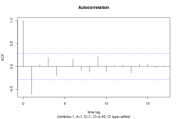
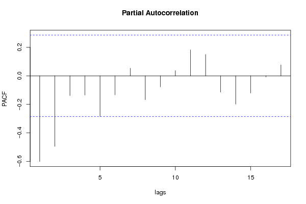
Title produced by software

(Partial) Autocorrelation Function

Date of computation

Mon, 05 Dec 2011 13:43:50 -0500

Cite this page as follows

Statistical Computations at FreeStatistics.org, Office for Research Development and Education, URL https://freestatistics.org/blog/index.php?v=date/2011/Dec/05/t13231106430e6ql9hw5jrue5m.htm/, Retrieved Fri, 03 May 2024 15:01:29 +0000

Statistical Computations at FreeStatistics.org, Office for Research Development and Education, URL https://freestatistics.org/blog/index.php?pk=151158, Retrieved Fri, 03 May 2024 15:01:29 +0000

QR Codes:

Paste this QR Code to cite your computation.

Original text written by user:

IsPrivate?

No (this computation is public)

User-defined keywords

Estimated Impact

150

Family? (F = Feedback message, R = changed R code, M = changed R Module, P = changed Parameters, D = changed Data)

-     [Univariate Explorative Data Analysis] [Run Sequence gebo...] [2008-12-12 13:32:37] [76963dc1903f0f612b6153510a3818cf]
- R  D  [Univariate Explorative Data Analysis] [Run Sequence gebo...] [2008-12-17 12:14:40] [76963dc1903f0f612b6153510a3818cf]
-         [Univariate Explorative Data Analysis] [Run Sequence Plot...] [2008-12-22 18:19:51] [1ce0d16c8f4225c977b42c8fa93bc163]
- RMP       [Univariate Data Series] [Identifying Integ...] [2009-11-22 12:08:06] [b98453cac15ba1066b407e146608df68]
- RMP         [(Partial) Autocorrelation Function] [Births] [2010-11-29 09:36:27] [b98453cac15ba1066b407e146608df68]
- R PD          [(Partial) Autocorrelation Function] [WS9 3.1 ACF d=0, D=0] [2010-12-07 10:00:49] [afe9379cca749d06b3d6872e02cc47ed]
- R  D            [(Partial) Autocorrelation Function] [ws9-2] [2011-12-05 18:26:48] [f7a862281046b7153543b12c78921b36]
-   P               [(Partial) Autocorrelation Function] [ws9-3] [2011-12-05 18:35:17] [f7a862281046b7153543b12c78921b36]
-   P                   [(Partial) Autocorrelation Function] [ws9-4] [2011-12-05 18:43:50] [47995d3a8fac585eeb070a274b466f8c] [Current]
-   P                     [(Partial) Autocorrelation Function] [ws9-4] [2011-12-05 18:46:25] [f7a862281046b7153543b12c78921b36] 
-   P                       [(Partial) Autocorrelation Function] [ws9-4] [2011-12-05 19:34:03] [f7a862281046b7153543b12c78921b36] 
-                             [(Partial) Autocorrelation Function] [ws9-4] [2011-12-05 19:35:13] [f7a862281046b7153543b12c78921b36] 
-  MP                           [(Partial) Autocorrelation Function] [paper2-3] [2011-12-21 20:49:59] [f7a862281046b7153543b12c78921b36] 

Feedback Forum

Post a new message

Dataseries X:

Download CSV

Histogram

Boxplots

Summary of computational transaction
Raw Input	view raw input (R code)
Raw Output	view raw output of R engine
Computing time	1 seconds
R Server	'Herman Ole Andreas Wold' @ wold.wessa.net

\begin{tabular}{lllllllll}
\hline
Summary of computational transaction \tabularnewline
Raw Input & view raw input (R code)  \tabularnewline
Raw Output & view raw output of R engine  \tabularnewline
Computing time & 1 seconds \tabularnewline
R Server & 'Herman Ole Andreas Wold' @ wold.wessa.net \tabularnewline
\hline
\end{tabular}
%Source: https://freestatistics.org/blog/index.php?pk=151158&T=0

[TABLE]
[ROW][C]Summary of computational transaction[/C][/ROW]
[ROW][C]Raw Input[/C][C]view raw input (R code) [/C][/ROW]
[ROW][C]Raw Output[/C][C]view raw output of R engine [/C][/ROW]
[ROW][C]Computing time[/C][C]1 seconds[/C][/ROW]
[ROW][C]R Server[/C][C]'Herman Ole Andreas Wold' @ wold.wessa.net[/C][/ROW]
[/TABLE]
Source: https://freestatistics.org/blog/index.php?pk=151158&T=0

Globally Unique Identifier (entire table): ba.freestatistics.org/blog/index.php?pk=151158&T=0

As an alternative you can also use a QR Code:

The GUIDs for individual cells are displayed in the table below:

Summary of computational transaction
Raw Input	view raw input (R code)
Raw Output	view raw output of R engine
Computing time	1 seconds
R Server	'Herman Ole Andreas Wold' @ wold.wessa.net

Autocorrelation Function
Time lag k	ACF(k)	T-STAT	P-value
1	-0.600777	-4.1187	7.7e-05
2	0.044663	0.3062	0.380405
3	0.190599	1.3067	0.098839
4	-0.19229	-1.3183	0.0969
5	-0.008319	-0.057	0.47738
6	0.164699	1.1291	0.132288
7	-0.080922	-0.5548	0.290841
8	-0.127147	-0.8717	0.193909
9	0.223016	1.5289	0.066493
10	-0.11512	-0.7892	0.216973
11	0.021214	0.1454	0.442495
12	0.039348	0.2698	0.394263
13	-0.141536	-0.9703	0.168427
14	0.060275	0.4132	0.340661
15	0.058659	0.4021	0.344699
16	-0.02026	-0.1389	0.445063
17	0.014856	0.1018	0.459655

\begin{tabular}{lllllllll}
\hline
Autocorrelation Function \tabularnewline
Time lag k & ACF(k) & T-STAT & P-value \tabularnewline
1 & -0.600777 & -4.1187 & 7.7e-05 \tabularnewline
2 & 0.044663 & 0.3062 & 0.380405 \tabularnewline
3 & 0.190599 & 1.3067 & 0.098839 \tabularnewline
4 & -0.19229 & -1.3183 & 0.0969 \tabularnewline
5 & -0.008319 & -0.057 & 0.47738 \tabularnewline
6 & 0.164699 & 1.1291 & 0.132288 \tabularnewline
7 & -0.080922 & -0.5548 & 0.290841 \tabularnewline
8 & -0.127147 & -0.8717 & 0.193909 \tabularnewline
9 & 0.223016 & 1.5289 & 0.066493 \tabularnewline
10 & -0.11512 & -0.7892 & 0.216973 \tabularnewline
11 & 0.021214 & 0.1454 & 0.442495 \tabularnewline
12 & 0.039348 & 0.2698 & 0.394263 \tabularnewline
13 & -0.141536 & -0.9703 & 0.168427 \tabularnewline
14 & 0.060275 & 0.4132 & 0.340661 \tabularnewline
15 & 0.058659 & 0.4021 & 0.344699 \tabularnewline
16 & -0.02026 & -0.1389 & 0.445063 \tabularnewline
17 & 0.014856 & 0.1018 & 0.459655 \tabularnewline
\hline
\end{tabular}
%Source: https://freestatistics.org/blog/index.php?pk=151158&T=1

[TABLE]
[ROW][C]Autocorrelation Function[/C][/ROW]
[ROW][C]Time lag k[/C][C]ACF(k)[/C][C]T-STAT[/C][C]P-value[/C][/ROW]
[ROW][C]1[/C][C]-0.600777[/C][C]-4.1187[/C][C]7.7e-05[/C][/ROW]
[ROW][C]2[/C][C]0.044663[/C][C]0.3062[/C][C]0.380405[/C][/ROW]
[ROW][C]3[/C][C]0.190599[/C][C]1.3067[/C][C]0.098839[/C][/ROW]
[ROW][C]4[/C][C]-0.19229[/C][C]-1.3183[/C][C]0.0969[/C][/ROW]
[ROW][C]5[/C][C]-0.008319[/C][C]-0.057[/C][C]0.47738[/C][/ROW]
[ROW][C]6[/C][C]0.164699[/C][C]1.1291[/C][C]0.132288[/C][/ROW]
[ROW][C]7[/C][C]-0.080922[/C][C]-0.5548[/C][C]0.290841[/C][/ROW]
[ROW][C]8[/C][C]-0.127147[/C][C]-0.8717[/C][C]0.193909[/C][/ROW]
[ROW][C]9[/C][C]0.223016[/C][C]1.5289[/C][C]0.066493[/C][/ROW]
[ROW][C]10[/C][C]-0.11512[/C][C]-0.7892[/C][C]0.216973[/C][/ROW]
[ROW][C]11[/C][C]0.021214[/C][C]0.1454[/C][C]0.442495[/C][/ROW]
[ROW][C]12[/C][C]0.039348[/C][C]0.2698[/C][C]0.394263[/C][/ROW]
[ROW][C]13[/C][C]-0.141536[/C][C]-0.9703[/C][C]0.168427[/C][/ROW]
[ROW][C]14[/C][C]0.060275[/C][C]0.4132[/C][C]0.340661[/C][/ROW]
[ROW][C]15[/C][C]0.058659[/C][C]0.4021[/C][C]0.344699[/C][/ROW]
[ROW][C]16[/C][C]-0.02026[/C][C]-0.1389[/C][C]0.445063[/C][/ROW]
[ROW][C]17[/C][C]0.014856[/C][C]0.1018[/C][C]0.459655[/C][/ROW]
[/TABLE]
Source: https://freestatistics.org/blog/index.php?pk=151158&T=1

Globally Unique Identifier (entire table): ba.freestatistics.org/blog/index.php?pk=151158&T=1

As an alternative you can also use a QR Code:

The GUIDs for individual cells are displayed in the table below:

Autocorrelation Function
Time lag k	ACF(k)	T-STAT	P-value
1	-0.600777	-4.1187	7.7e-05
2	0.044663	0.3062	0.380405
3	0.190599	1.3067	0.098839
4	-0.19229	-1.3183	0.0969
5	-0.008319	-0.057	0.47738
6	0.164699	1.1291	0.132288
7	-0.080922	-0.5548	0.290841
8	-0.127147	-0.8717	0.193909
9	0.223016	1.5289	0.066493
10	-0.11512	-0.7892	0.216973
11	0.021214	0.1454	0.442495
12	0.039348	0.2698	0.394263
13	-0.141536	-0.9703	0.168427
14	0.060275	0.4132	0.340661
15	0.058659	0.4021	0.344699
16	-0.02026	-0.1389	0.445063
17	0.014856	0.1018	0.459655

Partial Autocorrelation Function
Time lag k	PACF(k)	T-STAT	P-value
1	-0.600777	-4.1187	7.7e-05
2	-0.494894	-3.3928	0.000706
3	-0.138038	-0.9463	0.174408
4	-0.133901	-0.918	0.181658
5	-0.284933	-1.9534	0.02837
6	-0.133413	-0.9146	0.182526
7	0.05363	0.3677	0.357385
8	-0.166996	-1.1449	0.129031
9	-0.076823	-0.5267	0.30045
10	0.036715	0.2517	0.401182
11	0.182424	1.2506	0.108629
12	0.150622	1.0326	0.153535
13	-0.114015	-0.7816	0.219171
14	-0.198218	-1.3589	0.09033
15	-0.120749	-0.8278	0.205981
16	-0.007638	-0.0524	0.479229
17	0.076975	0.5277	0.300091

\begin{tabular}{lllllllll}
\hline
Partial Autocorrelation Function \tabularnewline
Time lag k & PACF(k) & T-STAT & P-value \tabularnewline
1 & -0.600777 & -4.1187 & 7.7e-05 \tabularnewline
2 & -0.494894 & -3.3928 & 0.000706 \tabularnewline
3 & -0.138038 & -0.9463 & 0.174408 \tabularnewline
4 & -0.133901 & -0.918 & 0.181658 \tabularnewline
5 & -0.284933 & -1.9534 & 0.02837 \tabularnewline
6 & -0.133413 & -0.9146 & 0.182526 \tabularnewline
7 & 0.05363 & 0.3677 & 0.357385 \tabularnewline
8 & -0.166996 & -1.1449 & 0.129031 \tabularnewline
9 & -0.076823 & -0.5267 & 0.30045 \tabularnewline
10 & 0.036715 & 0.2517 & 0.401182 \tabularnewline
11 & 0.182424 & 1.2506 & 0.108629 \tabularnewline
12 & 0.150622 & 1.0326 & 0.153535 \tabularnewline
13 & -0.114015 & -0.7816 & 0.219171 \tabularnewline
14 & -0.198218 & -1.3589 & 0.09033 \tabularnewline
15 & -0.120749 & -0.8278 & 0.205981 \tabularnewline
16 & -0.007638 & -0.0524 & 0.479229 \tabularnewline
17 & 0.076975 & 0.5277 & 0.300091 \tabularnewline
\hline
\end{tabular}
%Source: https://freestatistics.org/blog/index.php?pk=151158&T=2

[TABLE]
[ROW][C]Partial Autocorrelation Function[/C][/ROW]
[ROW][C]Time lag k[/C][C]PACF(k)[/C][C]T-STAT[/C][C]P-value[/C][/ROW]
[ROW][C]1[/C][C]-0.600777[/C][C]-4.1187[/C][C]7.7e-05[/C][/ROW]
[ROW][C]2[/C][C]-0.494894[/C][C]-3.3928[/C][C]0.000706[/C][/ROW]
[ROW][C]3[/C][C]-0.138038[/C][C]-0.9463[/C][C]0.174408[/C][/ROW]
[ROW][C]4[/C][C]-0.133901[/C][C]-0.918[/C][C]0.181658[/C][/ROW]
[ROW][C]5[/C][C]-0.284933[/C][C]-1.9534[/C][C]0.02837[/C][/ROW]
[ROW][C]6[/C][C]-0.133413[/C][C]-0.9146[/C][C]0.182526[/C][/ROW]
[ROW][C]7[/C][C]0.05363[/C][C]0.3677[/C][C]0.357385[/C][/ROW]
[ROW][C]8[/C][C]-0.166996[/C][C]-1.1449[/C][C]0.129031[/C][/ROW]
[ROW][C]9[/C][C]-0.076823[/C][C]-0.5267[/C][C]0.30045[/C][/ROW]
[ROW][C]10[/C][C]0.036715[/C][C]0.2517[/C][C]0.401182[/C][/ROW]
[ROW][C]11[/C][C]0.182424[/C][C]1.2506[/C][C]0.108629[/C][/ROW]
[ROW][C]12[/C][C]0.150622[/C][C]1.0326[/C][C]0.153535[/C][/ROW]
[ROW][C]13[/C][C]-0.114015[/C][C]-0.7816[/C][C]0.219171[/C][/ROW]
[ROW][C]14[/C][C]-0.198218[/C][C]-1.3589[/C][C]0.09033[/C][/ROW]
[ROW][C]15[/C][C]-0.120749[/C][C]-0.8278[/C][C]0.205981[/C][/ROW]
[ROW][C]16[/C][C]-0.007638[/C][C]-0.0524[/C][C]0.479229[/C][/ROW]
[ROW][C]17[/C][C]0.076975[/C][C]0.5277[/C][C]0.300091[/C][/ROW]
[/TABLE]
Source: https://freestatistics.org/blog/index.php?pk=151158&T=2

Globally Unique Identifier (entire table): ba.freestatistics.org/blog/index.php?pk=151158&T=2

As an alternative you can also use a QR Code:

The GUIDs for individual cells are displayed in the table below:

Partial Autocorrelation Function
Time lag k	PACF(k)	T-STAT	P-value
1	-0.600777	-4.1187	7.7e-05
2	-0.494894	-3.3928	0.000706
3	-0.138038	-0.9463	0.174408
4	-0.133901	-0.918	0.181658
5	-0.284933	-1.9534	0.02837
6	-0.133413	-0.9146	0.182526
7	0.05363	0.3677	0.357385
8	-0.166996	-1.1449	0.129031
9	-0.076823	-0.5267	0.30045
10	0.036715	0.2517	0.401182
11	0.182424	1.2506	0.108629
12	0.150622	1.0326	0.153535
13	-0.114015	-0.7816	0.219171
14	-0.198218	-1.3589	0.09033
15	-0.120749	-0.8278	0.205981
16	-0.007638	-0.0524	0.479229
17	0.076975	0.5277	0.300091

Figure 1

PNG link

Postscript link

PDF link

Figure 2

PNG link

Postscript link

PDF link

Parameters (Session):

par1 = Default ; par2 = 1 ; par3 = 1 ; par4 = 1 ; par5 = 12 ; par6 = White Noise ; par7 = 0.95 ;

Parameters (R input):

par1 = Default ; par2 = 1 ; par3 = 1 ; par4 = 1 ; par5 = 12 ; par6 = White Noise ; par7 = 0.95 ; par8 = ;

R code (references can be found in the software module):

if (par1 == 'Default') {
par1 = 10*log10(length(x))
} else {
par1 <- as.numeric(par1)
}
par2 <- as.numeric(par2)
par3 <- as.numeric(par3)
par4 <- as.numeric(par4)
par5 <- as.numeric(par5)
if (par6 == 'White Noise') par6 <- 'white' else par6 <- 'ma'
par7 <- as.numeric(par7)
if (par2 == 0) {
x <- log(x)
} else {
x <- (x ^ par2 - 1) / par2
}
if (par3 > 0) x <- diff(x,lag=1,difference=par3)
if (par4 > 0) x <- diff(x,lag=par5,difference=par4)
bitmap(file='pic1.png')
racf <- acf(x, par1, main='Autocorrelation', xlab='time lag', ylab='ACF', ci.type=par6, ci=par7, sub=paste('(lambda=',par2,', d=',par3,', D=',par4,', CI=', par7, ', CI type=',par6,')',sep=''))
dev.off()
bitmap(file='pic2.png')
rpacf <- pacf(x,par1,main='Partial Autocorrelation',xlab='lags',ylab='PACF')
dev.off()
(myacf <- c(racf$acf))
(mypacf <- c(rpacf$acf))
lengthx <- length(x)
sqrtn <- sqrt(lengthx)
load(file='createtable')
a<-table.start()
a<-table.row.start(a)
a<-table.element(a,'Autocorrelation Function',4,TRUE)
a<-table.row.end(a)
a<-table.row.start(a)
a<-table.element(a,'Time lag k',header=TRUE)
a<-table.element(a,hyperlink('basics.htm','ACF(k)','click here for more information about the Autocorrelation Function'),header=TRUE)
a<-table.element(a,'T-STAT',header=TRUE)
a<-table.element(a,'P-value',header=TRUE)
a<-table.row.end(a)
for (i in 2:(par1+1)) {
a<-table.row.start(a)
a<-table.element(a,i-1,header=TRUE)
a<-table.element(a,round(myacf[i],6))
mytstat <- myacf[i]*sqrtn
a<-table.element(a,round(mytstat,4))
a<-table.element(a,round(1-pt(abs(mytstat),lengthx),6))
a<-table.row.end(a)
}
a<-table.end(a)
table.save(a,file='mytable.tab')
a<-table.start()
a<-table.row.start(a)
a<-table.element(a,'Partial Autocorrelation Function',4,TRUE)
a<-table.row.end(a)
a<-table.row.start(a)
a<-table.element(a,'Time lag k',header=TRUE)
a<-table.element(a,hyperlink('basics.htm','PACF(k)','click here for more information about the Partial Autocorrelation Function'),header=TRUE)
a<-table.element(a,'T-STAT',header=TRUE)
a<-table.element(a,'P-value',header=TRUE)
a<-table.row.end(a)
for (i in 1:par1) {
a<-table.row.start(a)
a<-table.element(a,i,header=TRUE)
a<-table.element(a,round(mypacf[i],6))
mytstat <- mypacf[i]*sqrtn
a<-table.element(a,round(mytstat,4))
a<-table.element(a,round(1-pt(abs(mytstat),lengthx),6))
a<-table.row.end(a)
}
a<-table.end(a)
table.save(a,file='mytable1.tab')

Free Statistics

Description of Statistical Computation

Tree of Dependent Computations

Dataset

Tables (Output of Computation)

Figures (Output of Computation)

Input Parameters & R Code