Free Statistics
of Irreproducible Research!
Description of Statistical Computation | |||||||||||||||||||||||||||||||||||||||||||||||||||||||||||||||||||||||||||||||||
|---|---|---|---|---|---|---|---|---|---|---|---|---|---|---|---|---|---|---|---|---|---|---|---|---|---|---|---|---|---|---|---|---|---|---|---|---|---|---|---|---|---|---|---|---|---|---|---|---|---|---|---|---|---|---|---|---|---|---|---|---|---|---|---|---|---|---|---|---|---|---|---|---|---|---|---|---|---|---|---|---|---|
| Author's title | |||||||||||||||||||||||||||||||||||||||||||||||||||||||||||||||||||||||||||||||||
| Author | *Unverified author* | ||||||||||||||||||||||||||||||||||||||||||||||||||||||||||||||||||||||||||||||||
| R Software Module | rwasp_bootstrapplot.wasp | ||||||||||||||||||||||||||||||||||||||||||||||||||||||||||||||||||||||||||||||||
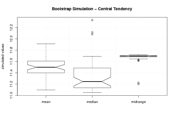
| Title produced by software | Blocked Bootstrap Plot - Central Tendency | ||||||||||||||||||||||||||||||||||||||||||||||||||||||||||||||||||||||||||||||||
| Date of computation | Sun, 04 Dec 2011 13:09:38 -0500 | ||||||||||||||||||||||||||||||||||||||||||||||||||||||||||||||||||||||||||||||||
| Cite this page as follows | Statistical Computations at FreeStatistics.org, Office for Research Development and Education, URL https://freestatistics.org/blog/index.php?v=date/2011/Dec/04/t132302224667dtmd1t1214w01.htm/, Retrieved Sun, 05 May 2024 12:37:55 +0000 | ||||||||||||||||||||||||||||||||||||||||||||||||||||||||||||||||||||||||||||||||
| Statistical Computations at FreeStatistics.org, Office for Research Development and Education, URL https://freestatistics.org/blog/index.php?pk=150720, Retrieved Sun, 05 May 2024 12:37:55 +0000 | |||||||||||||||||||||||||||||||||||||||||||||||||||||||||||||||||||||||||||||||||
| QR Codes: | |||||||||||||||||||||||||||||||||||||||||||||||||||||||||||||||||||||||||||||||||
|
| |||||||||||||||||||||||||||||||||||||||||||||||||||||||||||||||||||||||||||||||||
| Original text written by user: | |||||||||||||||||||||||||||||||||||||||||||||||||||||||||||||||||||||||||||||||||
| IsPrivate? | No (this computation is public) | ||||||||||||||||||||||||||||||||||||||||||||||||||||||||||||||||||||||||||||||||
| User-defined keywords | KDGP2W22 | ||||||||||||||||||||||||||||||||||||||||||||||||||||||||||||||||||||||||||||||||
| Estimated Impact | 102 | ||||||||||||||||||||||||||||||||||||||||||||||||||||||||||||||||||||||||||||||||
Tree of Dependent Computations | |||||||||||||||||||||||||||||||||||||||||||||||||||||||||||||||||||||||||||||||||
| Family? (F = Feedback message, R = changed R code, M = changed R Module, P = changed Parameters, D = changed Data) | |||||||||||||||||||||||||||||||||||||||||||||||||||||||||||||||||||||||||||||||||
| - [Blocked Bootstrap Plot - Central Tendency] [Evolutie gemiddel...] [2011-12-04 18:09:38] [9b00bb73e1719a6b710100764835da33] [Current] - PD [Blocked Bootstrap Plot - Central Tendency] [e] [2011-12-04 18:12:29] [d700a6813b2ef07b7398fe84f8eae4b7] - PD [Blocked Bootstrap Plot - Central Tendency] [Evolutie gemiddel...] [2011-12-04 18:12:29] [d700a6813b2ef07b7398fe84f8eae4b7] - PD [Blocked Bootstrap Plot - Central Tendency] [Evolutie gemiddel...] [2011-12-04 18:15:16] [d700a6813b2ef07b7398fe84f8eae4b7] - RMPD [Variability] [Maximumprijs show...] [2011-12-04 18:29:37] [d700a6813b2ef07b7398fe84f8eae4b7] - RMPD [Standard Deviation Plot] [Inschrijvingen ni...] [2011-12-04 18:35:36] [d700a6813b2ef07b7398fe84f8eae4b7] - RMPD [Standard Deviation-Mean Plot] [Inschrijvingen ni...] [2011-12-04 18:44:52] [d700a6813b2ef07b7398fe84f8eae4b7] - R P [Standard Deviation-Mean Plot] [KDGP2W82] [2011-12-11 13:00:18] [d700a6813b2ef07b7398fe84f8eae4b7] - [Standard Deviation-Mean Plot] [KDGP2W83] [2011-12-11 13:08:30] [ed108f6919ebadc8e809f8b86ef40b05] - RMP [Classical Decomposition] [KDGP2W91] [2011-12-11 13:28:26] [d700a6813b2ef07b7398fe84f8eae4b7] - R [Classical Decomposition] [] [2011-12-11 13:41:56] [d700a6813b2ef07b7398fe84f8eae4b7] - RMPD [Classical Decomposition] [] [2011-12-11 13:38:04] [d700a6813b2ef07b7398fe84f8eae4b7] - [Standard Deviation-Mean Plot] [Inschrijvingen ni...] [2011-12-11 13:46:28] [d700a6813b2ef07b7398fe84f8eae4b7] - RMP [Variability] [Evolutie gemiddel...] [2011-12-04 19:01:51] [d700a6813b2ef07b7398fe84f8eae4b7] - RMPD [Standard Deviation Plot] [Evolutie gemiddel...] [2011-12-04 19:05:18] [d700a6813b2ef07b7398fe84f8eae4b7] - RMPD [Standard Deviation-Mean Plot] [Evolutie gemiddel...] [2011-12-04 19:11:32] [d700a6813b2ef07b7398fe84f8eae4b7] - R P [Standard Deviation-Mean Plot] [KDGP2W83] [2011-12-11 13:11:58] [d700a6813b2ef07b7398fe84f8eae4b7] - [Standard Deviation-Mean Plot] [Evolutie gemiddel...] [2011-12-11 13:44:08] [d700a6813b2ef07b7398fe84f8eae4b7] | |||||||||||||||||||||||||||||||||||||||||||||||||||||||||||||||||||||||||||||||||
| Feedback Forum | |||||||||||||||||||||||||||||||||||||||||||||||||||||||||||||||||||||||||||||||||
Post a new message | |||||||||||||||||||||||||||||||||||||||||||||||||||||||||||||||||||||||||||||||||
Dataset | |||||||||||||||||||||||||||||||||||||||||||||||||||||||||||||||||||||||||||||||||
| Dataseries X: | |||||||||||||||||||||||||||||||||||||||||||||||||||||||||||||||||||||||||||||||||
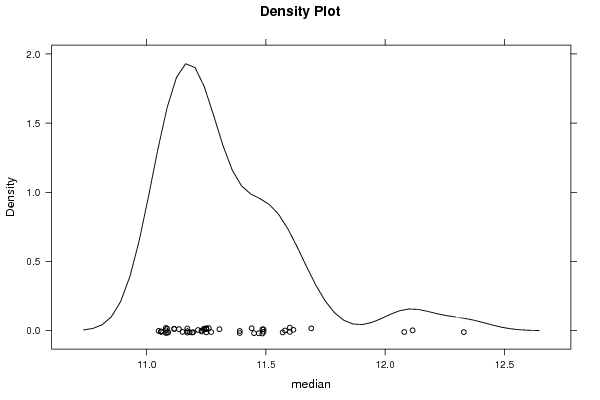
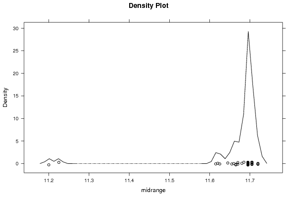
10,93 10,92 10,89 10,94 10,98 10,99 11,02 11,04 11,05 11,05 11,02 10,91 11,01 11,02 11,03 11,04 11,06 11,08 11,06 11,06 11,09 11,07 11,06 11,08 11,08 11,08 11,11 11,09 11,08 11,05 11,07 11,06 11,06 11,07 11,02 11,01 11,04 11,02 11,03 11,17 11,19 11,15 11,13 11,06 11,01 11,03 10,99 10,94 11 11,06 11,06 11,05 11,04 11,15 11,2 11,16 11,3 11,23 11,25 11,25 11,12 11,14 11,17 11,25 11,27 11,34 11,39 11,44 11,46 11,49 11,51 11,48 11,49 11,52 11,56 11,58 11,58 11,58 11,6 11,62 11,62 11,64 11,67 11,66 11,72 11,82 11,9 12,04 12,08 12,15 12,19 12,22 12,23 12,25 12,26 12,27 12,34 12,38 12,42 12,43 12,48 12,5 12,5 12,49 12,46 12,45 12,45 12,38 12,42 12,37 12,35 12,35 12,36 12,32 12,32 12,34 12,35 12,34 12,31 12,24 | |||||||||||||||||||||||||||||||||||||||||||||||||||||||||||||||||||||||||||||||||
Tables (Output of Computation) | |||||||||||||||||||||||||||||||||||||||||||||||||||||||||||||||||||||||||||||||||
| |||||||||||||||||||||||||||||||||||||||||||||||||||||||||||||||||||||||||||||||||
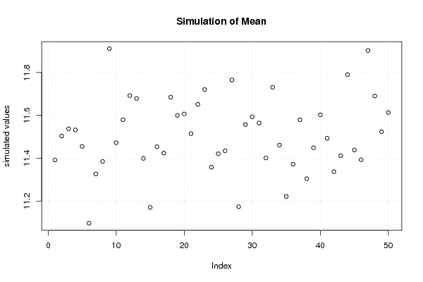
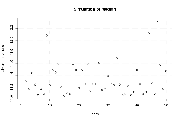
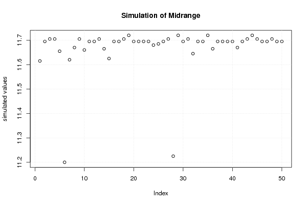
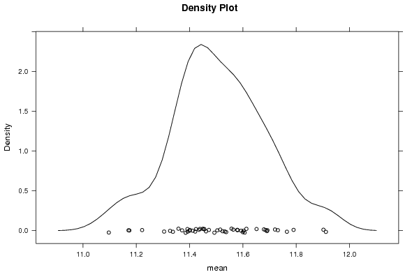
Figures (Output of Computation) | |||||||||||||||||||||||||||||||||||||||||||||||||||||||||||||||||||||||||||||||||
Input Parameters & R Code | |||||||||||||||||||||||||||||||||||||||||||||||||||||||||||||||||||||||||||||||||
| Parameters (Session): | |||||||||||||||||||||||||||||||||||||||||||||||||||||||||||||||||||||||||||||||||
| par1 = 50 ; par2 = 12 ; | |||||||||||||||||||||||||||||||||||||||||||||||||||||||||||||||||||||||||||||||||
| Parameters (R input): | |||||||||||||||||||||||||||||||||||||||||||||||||||||||||||||||||||||||||||||||||
| par1 = 50 ; par2 = 12 ; | |||||||||||||||||||||||||||||||||||||||||||||||||||||||||||||||||||||||||||||||||
| R code (references can be found in the software module): | |||||||||||||||||||||||||||||||||||||||||||||||||||||||||||||||||||||||||||||||||
par1 <- as.numeric(par1) | |||||||||||||||||||||||||||||||||||||||||||||||||||||||||||||||||||||||||||||||||