Free Statistics
of Irreproducible Research!
Description of Statistical Computation | |||||||||||||||||||||||||||||||||||||||||||||||||||||
|---|---|---|---|---|---|---|---|---|---|---|---|---|---|---|---|---|---|---|---|---|---|---|---|---|---|---|---|---|---|---|---|---|---|---|---|---|---|---|---|---|---|---|---|---|---|---|---|---|---|---|---|---|---|
| Author's title | |||||||||||||||||||||||||||||||||||||||||||||||||||||
| Author | *Unverified author* | ||||||||||||||||||||||||||||||||||||||||||||||||||||
| R Software Module | rwasp_edauni.wasp | ||||||||||||||||||||||||||||||||||||||||||||||||||||
| Title produced by software | Univariate Explorative Data Analysis | ||||||||||||||||||||||||||||||||||||||||||||||||||||
| Date of computation | Sat, 03 Dec 2011 07:45:00 -0500 | ||||||||||||||||||||||||||||||||||||||||||||||||||||
| Cite this page as follows | Statistical Computations at FreeStatistics.org, Office for Research Development and Education, URL https://freestatistics.org/blog/index.php?v=date/2011/Dec/03/t13229163255pf4b47sg4yyuh7.htm/, Retrieved Thu, 03 Jul 2025 08:35:28 +0000 | ||||||||||||||||||||||||||||||||||||||||||||||||||||
| Statistical Computations at FreeStatistics.org, Office for Research Development and Education, URL https://freestatistics.org/blog/index.php?pk=150434, Retrieved Thu, 03 Jul 2025 08:35:28 +0000 | |||||||||||||||||||||||||||||||||||||||||||||||||||||
| QR Codes: | |||||||||||||||||||||||||||||||||||||||||||||||||||||
|
| |||||||||||||||||||||||||||||||||||||||||||||||||||||
| Original text written by user: | |||||||||||||||||||||||||||||||||||||||||||||||||||||
| IsPrivate? | No (this computation is public) | ||||||||||||||||||||||||||||||||||||||||||||||||||||
| User-defined keywords | |||||||||||||||||||||||||||||||||||||||||||||||||||||
| Estimated Impact | 230 | ||||||||||||||||||||||||||||||||||||||||||||||||||||
Tree of Dependent Computations | |||||||||||||||||||||||||||||||||||||||||||||||||||||
| Family? (F = Feedback message, R = changed R code, M = changed R Module, P = changed Parameters, D = changed Data) | |||||||||||||||||||||||||||||||||||||||||||||||||||||
| - [Bivariate Data Series] [Bivariate dataset] [2008-01-05 23:51:08] [74be16979710d4c4e7c6647856088456] - RMPD [Univariate Explorative Data Analysis] [SHW_WS4_Q3] [2009-10-23 09:32:44] [8b1aef4e7013bd33fbc2a5833375c5f5] - M D [Univariate Explorative Data Analysis] [Paper Regressie A...] [2010-12-03 21:58:57] [814f53995537cd15c528d8efbf1cf544] - R D [Univariate Explorative Data Analysis] [] [2011-12-03 12:45:00] [d41d8cd98f00b204e9800998ecf8427e] [Current] | |||||||||||||||||||||||||||||||||||||||||||||||||||||
| Feedback Forum | |||||||||||||||||||||||||||||||||||||||||||||||||||||
Post a new message | |||||||||||||||||||||||||||||||||||||||||||||||||||||
Dataset | |||||||||||||||||||||||||||||||||||||||||||||||||||||
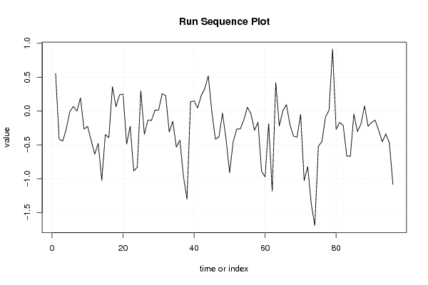
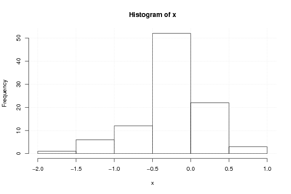
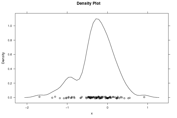
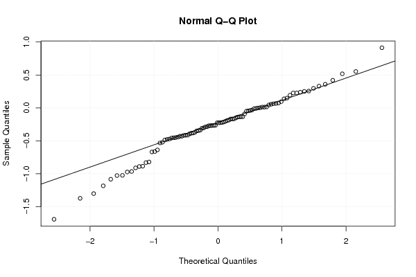
| Dataseries X: | |||||||||||||||||||||||||||||||||||||||||||||||||||||
0,552514900 -0,415233631 -0,443505270 -0,269121643 -0,008403113 0,067701517 -0,001956584 0,192909884 -0,267874375 -0,226255248 -0,430298473 -0,638100667 -0,479124765 -1,024474510 -0,348637834 -0,393955343 0,358931095 0,063381185 0,238243996 0,250678752 -0,487515927 -0,225775256 -0,885760418 -0,830655282 0,296897628 -0,344915585 -0,133869039 -0,139756916 0,014602114 0,011865030 0,255115762 0,226820722 -0,309023585 -0,151618802 -0,531858288 -0,429638741 -0,965975558 -1,301831527 0,137422114 0,148700147 0,044143121 0,226631056 0,330163975 0,517790690 -0,011123165 -0,416908592 -0,381488696 -0,031884958 -0,414393439 -0,911095332 -0,457371141 -0,266401460 -0,263471321 -0,134106783 0,055333648 -0,039713557 -0,285383350 -0,167483970 -0,890023318 -0,973150900 -0,185793746 -1,183720382 0,419787663 -0,220470559 0,002758416 0,094605253 -0,203747577 -0,370446898 -0,384431401 -0,050166061 -1,027647092 -0,821409393 -1,373356682 -1,691725416 -0,521561774 -0,449977604 -0,090629713 0,011651815 0,913398739 -0,271811435 -0,168925538 -0,213969528 -0,663331231 -0,668861966 -0,045192980 -0,304069160 -0,190343886 0,074887422 -0,225243865 -0,167614301 -0,135891117 -0,289021535 -0,454125093 -0,337581704 -0,472963398 -1,083843021 | |||||||||||||||||||||||||||||||||||||||||||||||||||||
Tables (Output of Computation) | |||||||||||||||||||||||||||||||||||||||||||||||||||||
| |||||||||||||||||||||||||||||||||||||||||||||||||||||
Figures (Output of Computation) | |||||||||||||||||||||||||||||||||||||||||||||||||||||
Input Parameters & R Code | |||||||||||||||||||||||||||||||||||||||||||||||||||||
| Parameters (Session): | |||||||||||||||||||||||||||||||||||||||||||||||||||||
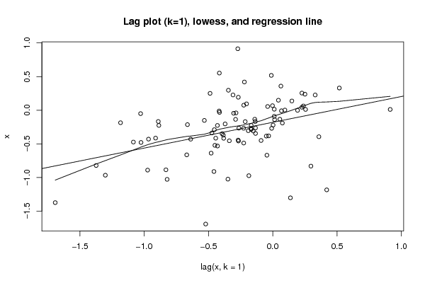
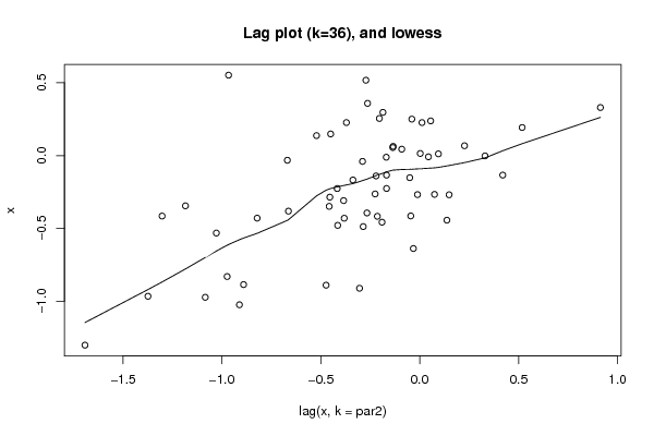
| par1 = 0 ; par2 = 36 ; | |||||||||||||||||||||||||||||||||||||||||||||||||||||
| Parameters (R input): | |||||||||||||||||||||||||||||||||||||||||||||||||||||
| par1 = 0 ; par2 = 36 ; | |||||||||||||||||||||||||||||||||||||||||||||||||||||
| R code (references can be found in the software module): | |||||||||||||||||||||||||||||||||||||||||||||||||||||
par1 <- as.numeric(par1) | |||||||||||||||||||||||||||||||||||||||||||||||||||||