Repository of Reproducible Computations

Free Statistics

of Irreproducible Research!

Author's title

Author

*Unverified author*

R Software Module

rwasp_arimaforecasting.wasp

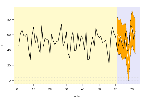
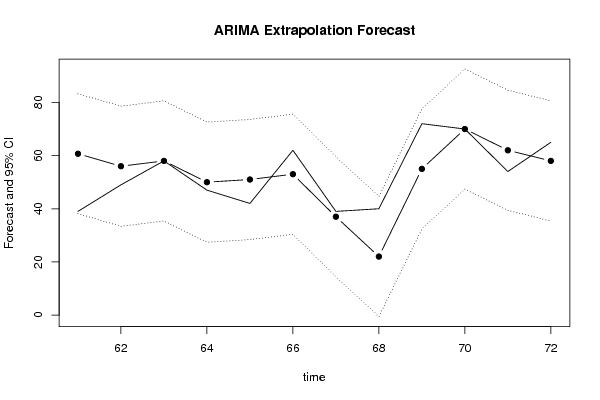
Title produced by software

ARIMA Forecasting

Date of computation

Sat, 03 Dec 2011 05:54:00 -0500

Cite this page as follows

Statistical Computations at FreeStatistics.org, Office for Research Development and Education, URL https://freestatistics.org/blog/index.php?v=date/2011/Dec/03/t1322909705d63h2cskvkybc4h.htm/, Retrieved Sun, 28 Apr 2024 21:26:28 +0000

Statistical Computations at FreeStatistics.org, Office for Research Development and Education, URL https://freestatistics.org/blog/index.php?pk=150399, Retrieved Sun, 28 Apr 2024 21:26:28 +0000

QR Codes:

Paste this QR Code to cite your computation.

Original text written by user:

IsPrivate?

No (this computation is public)

User-defined keywords

Estimated Impact

152

Family? (F = Feedback message, R = changed R code, M = changed R Module, P = changed Parameters, D = changed Data)

-     [Univariate Data Series] [data set] [2008-12-01 19:54:57] [b98453cac15ba1066b407e146608df68]
- RMP   [Standard Deviation-Mean Plot] [Unemployment] [2010-11-29 10:34:47] [b98453cac15ba1066b407e146608df68]
- RMP     [ARIMA Forecasting] [Unemployment] [2010-11-29 20:46:45] [b98453cac15ba1066b407e146608df68]
-    D      [ARIMA Forecasting] [WS 9 Forecasting ...] [2010-12-03 22:01:04] [8081b8996d5947580de3eb171e82db4f]
-   PD        [ARIMA Forecasting] [Workshop 9, Forecast] [2010-12-05 20:21:31] [3635fb7041b1998c5a1332cf9de22bce]
-   P           [ARIMA Forecasting] [ARIMA Extrapolati...] [2010-12-06 22:58:10] [3635fb7041b1998c5a1332cf9de22bce]
-   P             [ARIMA Forecasting] [Verbetering WS9] [2010-12-14 19:20:19] [3635fb7041b1998c5a1332cf9de22bce]
- R PD                [ARIMA Forecasting] [WS9 ARIMA forecas...] [2011-12-03 10:54:00] [d41d8cd98f00b204e9800998ecf8427e] [Current]
- R PD                  [ARIMA Forecasting] [paper] [2011-12-20 18:16:40] [43239ed98a62e091c70785d80176537f] 

Feedback Forum

Post a new message

Dataseries X:

Download CSV

Histogram

Boxplots

Summary of computational transaction
Raw Input	view raw input (R code)
Raw Output	view raw output of R engine
Computing time	2 seconds
R Server	'AstonUniversity' @ aston.wessa.net

\begin{tabular}{lllllllll}
\hline
Summary of computational transaction \tabularnewline
Raw Input & view raw input (R code)  \tabularnewline
Raw Output & view raw output of R engine  \tabularnewline
Computing time & 2 seconds \tabularnewline
R Server & 'AstonUniversity' @ aston.wessa.net \tabularnewline
\hline
\end{tabular}
%Source: https://freestatistics.org/blog/index.php?pk=150399&T=0

[TABLE]
[ROW][C]Summary of computational transaction[/C][/ROW]
[ROW][C]Raw Input[/C][C]view raw input (R code) [/C][/ROW]
[ROW][C]Raw Output[/C][C]view raw output of R engine [/C][/ROW]
[ROW][C]Computing time[/C][C]2 seconds[/C][/ROW]
[ROW][C]R Server[/C][C]'AstonUniversity' @ aston.wessa.net[/C][/ROW]
[/TABLE]
Source: https://freestatistics.org/blog/index.php?pk=150399&T=0

Globally Unique Identifier (entire table): ba.freestatistics.org/blog/index.php?pk=150399&T=0

As an alternative you can also use a QR Code:

The GUIDs for individual cells are displayed in the table below:

Summary of computational transaction
Raw Input	view raw input (R code)
Raw Output	view raw output of R engine
Computing time	2 seconds
R Server	'AstonUniversity' @ aston.wessa.net

Univariate ARIMA Extrapolation Forecast
time	Y[t]	F[t]	95% LB	95% UB	p-value(H0: Y[t] = F[t])	P(F[t]>Y[t-1])	P(F[t]>Y[t-s])	P(F[t]>Y[60])
48	69	-	-	-	-	-	-	-
49	60	-	-	-	-	-	-	-
50	56	-	-	-	-	-	-	-
51	58	-	-	-	-	-	-	-
52	50	-	-	-	-	-	-	-
53	51	-	-	-	-	-	-	-
54	53	-	-	-	-	-	-	-
55	37	-	-	-	-	-	-	-
56	22	-	-	-	-	-	-	-
57	55	-	-	-	-	-	-	-
58	70	-	-	-	-	-	-	-
59	62	-	-	-	-	-	-	-
60	58	-	-	-	-	-	-	-
61	39	60.6978	38.1515	83.2441	0.0296	0.5927	0.5242	0.5927
62	49	56	33.3955	78.6045	0.2719	0.9298	0.5	0.4312
63	58	58	35.3955	80.6045	0.5	0.7824	0.5	0.5
64	47	50	27.3955	72.6045	0.3974	0.2439	0.5	0.2439
65	42	51	28.3955	73.6045	0.2176	0.6356	0.5	0.2719
66	62	53	30.3955	75.6045	0.2176	0.8299	0.5	0.3323
67	39	37	14.3955	59.6045	0.4312	0.0151	0.5	0.0343
68	40	22	-0.6045	44.6045	0.0593	0.0702	0.5	9e-04
69	72	55	32.3955	77.6045	0.0702	0.9033	0.5	0.3974
70	70	70	47.3955	92.6045	0.5	0.4312	0.5	0.8509
71	54	62	39.3955	84.6045	0.2439	0.2439	0.5	0.6356
72	65	58	35.3955	80.6045	0.2719	0.6356	0.5	0.5

\begin{tabular}{lllllllll}
\hline
Univariate ARIMA Extrapolation Forecast \tabularnewline
time & Y[t] & F[t] & 95% LB & 95% UB & p-value(H0: Y[t] = F[t]) & P(F[t]>Y[t-1]) & P(F[t]>Y[t-s]) & P(F[t]>Y[60]) \tabularnewline
48 & 69 & - & - & - & - & - & - & - \tabularnewline
49 & 60 & - & - & - & - & - & - & - \tabularnewline
50 & 56 & - & - & - & - & - & - & - \tabularnewline
51 & 58 & - & - & - & - & - & - & - \tabularnewline
52 & 50 & - & - & - & - & - & - & - \tabularnewline
53 & 51 & - & - & - & - & - & - & - \tabularnewline
54 & 53 & - & - & - & - & - & - & - \tabularnewline
55 & 37 & - & - & - & - & - & - & - \tabularnewline
56 & 22 & - & - & - & - & - & - & - \tabularnewline
57 & 55 & - & - & - & - & - & - & - \tabularnewline
58 & 70 & - & - & - & - & - & - & - \tabularnewline
59 & 62 & - & - & - & - & - & - & - \tabularnewline
60 & 58 & - & - & - & - & - & - & - \tabularnewline
61 & 39 & 60.6978 & 38.1515 & 83.2441 & 0.0296 & 0.5927 & 0.5242 & 0.5927 \tabularnewline
62 & 49 & 56 & 33.3955 & 78.6045 & 0.2719 & 0.9298 & 0.5 & 0.4312 \tabularnewline
63 & 58 & 58 & 35.3955 & 80.6045 & 0.5 & 0.7824 & 0.5 & 0.5 \tabularnewline
64 & 47 & 50 & 27.3955 & 72.6045 & 0.3974 & 0.2439 & 0.5 & 0.2439 \tabularnewline
65 & 42 & 51 & 28.3955 & 73.6045 & 0.2176 & 0.6356 & 0.5 & 0.2719 \tabularnewline
66 & 62 & 53 & 30.3955 & 75.6045 & 0.2176 & 0.8299 & 0.5 & 0.3323 \tabularnewline
67 & 39 & 37 & 14.3955 & 59.6045 & 0.4312 & 0.0151 & 0.5 & 0.0343 \tabularnewline
68 & 40 & 22 & -0.6045 & 44.6045 & 0.0593 & 0.0702 & 0.5 & 9e-04 \tabularnewline
69 & 72 & 55 & 32.3955 & 77.6045 & 0.0702 & 0.9033 & 0.5 & 0.3974 \tabularnewline
70 & 70 & 70 & 47.3955 & 92.6045 & 0.5 & 0.4312 & 0.5 & 0.8509 \tabularnewline
71 & 54 & 62 & 39.3955 & 84.6045 & 0.2439 & 0.2439 & 0.5 & 0.6356 \tabularnewline
72 & 65 & 58 & 35.3955 & 80.6045 & 0.2719 & 0.6356 & 0.5 & 0.5 \tabularnewline
\hline
\end{tabular}
%Source: https://freestatistics.org/blog/index.php?pk=150399&T=1

[TABLE]
[ROW][C]Univariate ARIMA Extrapolation Forecast[/C][/ROW]
[ROW][C]time[/C][C]Y[t][/C][C]F[t][/C][C]95% LB[/C][C]95% UB[/C][C]p-value(H0: Y[t] = F[t])[/C][C]P(F[t]>Y[t-1])[/C][C]P(F[t]>Y[t-s])[/C][C]P(F[t]>Y[60])[/C][/ROW]
[ROW][C]48[/C][C]69[/C][C]-[/C][C]-[/C][C]-[/C][C]-[/C][C]-[/C][C]-[/C][C]-[/C][/ROW]
[ROW][C]49[/C][C]60[/C][C]-[/C][C]-[/C][C]-[/C][C]-[/C][C]-[/C][C]-[/C][C]-[/C][/ROW]
[ROW][C]50[/C][C]56[/C][C]-[/C][C]-[/C][C]-[/C][C]-[/C][C]-[/C][C]-[/C][C]-[/C][/ROW]
[ROW][C]51[/C][C]58[/C][C]-[/C][C]-[/C][C]-[/C][C]-[/C][C]-[/C][C]-[/C][C]-[/C][/ROW]
[ROW][C]52[/C][C]50[/C][C]-[/C][C]-[/C][C]-[/C][C]-[/C][C]-[/C][C]-[/C][C]-[/C][/ROW]
[ROW][C]53[/C][C]51[/C][C]-[/C][C]-[/C][C]-[/C][C]-[/C][C]-[/C][C]-[/C][C]-[/C][/ROW]
[ROW][C]54[/C][C]53[/C][C]-[/C][C]-[/C][C]-[/C][C]-[/C][C]-[/C][C]-[/C][C]-[/C][/ROW]
[ROW][C]55[/C][C]37[/C][C]-[/C][C]-[/C][C]-[/C][C]-[/C][C]-[/C][C]-[/C][C]-[/C][/ROW]
[ROW][C]56[/C][C]22[/C][C]-[/C][C]-[/C][C]-[/C][C]-[/C][C]-[/C][C]-[/C][C]-[/C][/ROW]
[ROW][C]57[/C][C]55[/C][C]-[/C][C]-[/C][C]-[/C][C]-[/C][C]-[/C][C]-[/C][C]-[/C][/ROW]
[ROW][C]58[/C][C]70[/C][C]-[/C][C]-[/C][C]-[/C][C]-[/C][C]-[/C][C]-[/C][C]-[/C][/ROW]
[ROW][C]59[/C][C]62[/C][C]-[/C][C]-[/C][C]-[/C][C]-[/C][C]-[/C][C]-[/C][C]-[/C][/ROW]
[ROW][C]60[/C][C]58[/C][C]-[/C][C]-[/C][C]-[/C][C]-[/C][C]-[/C][C]-[/C][C]-[/C][/ROW]
[ROW][C]61[/C][C]39[/C][C]60.6978[/C][C]38.1515[/C][C]83.2441[/C][C]0.0296[/C][C]0.5927[/C][C]0.5242[/C][C]0.5927[/C][/ROW]
[ROW][C]62[/C][C]49[/C][C]56[/C][C]33.3955[/C][C]78.6045[/C][C]0.2719[/C][C]0.9298[/C][C]0.5[/C][C]0.4312[/C][/ROW]
[ROW][C]63[/C][C]58[/C][C]58[/C][C]35.3955[/C][C]80.6045[/C][C]0.5[/C][C]0.7824[/C][C]0.5[/C][C]0.5[/C][/ROW]
[ROW][C]64[/C][C]47[/C][C]50[/C][C]27.3955[/C][C]72.6045[/C][C]0.3974[/C][C]0.2439[/C][C]0.5[/C][C]0.2439[/C][/ROW]
[ROW][C]65[/C][C]42[/C][C]51[/C][C]28.3955[/C][C]73.6045[/C][C]0.2176[/C][C]0.6356[/C][C]0.5[/C][C]0.2719[/C][/ROW]
[ROW][C]66[/C][C]62[/C][C]53[/C][C]30.3955[/C][C]75.6045[/C][C]0.2176[/C][C]0.8299[/C][C]0.5[/C][C]0.3323[/C][/ROW]
[ROW][C]67[/C][C]39[/C][C]37[/C][C]14.3955[/C][C]59.6045[/C][C]0.4312[/C][C]0.0151[/C][C]0.5[/C][C]0.0343[/C][/ROW]
[ROW][C]68[/C][C]40[/C][C]22[/C][C]-0.6045[/C][C]44.6045[/C][C]0.0593[/C][C]0.0702[/C][C]0.5[/C][C]9e-04[/C][/ROW]
[ROW][C]69[/C][C]72[/C][C]55[/C][C]32.3955[/C][C]77.6045[/C][C]0.0702[/C][C]0.9033[/C][C]0.5[/C][C]0.3974[/C][/ROW]
[ROW][C]70[/C][C]70[/C][C]70[/C][C]47.3955[/C][C]92.6045[/C][C]0.5[/C][C]0.4312[/C][C]0.5[/C][C]0.8509[/C][/ROW]
[ROW][C]71[/C][C]54[/C][C]62[/C][C]39.3955[/C][C]84.6045[/C][C]0.2439[/C][C]0.2439[/C][C]0.5[/C][C]0.6356[/C][/ROW]
[ROW][C]72[/C][C]65[/C][C]58[/C][C]35.3955[/C][C]80.6045[/C][C]0.2719[/C][C]0.6356[/C][C]0.5[/C][C]0.5[/C][/ROW]
[/TABLE]
Source: https://freestatistics.org/blog/index.php?pk=150399&T=1

Globally Unique Identifier (entire table): ba.freestatistics.org/blog/index.php?pk=150399&T=1

As an alternative you can also use a QR Code:

The GUIDs for individual cells are displayed in the table below:

Univariate ARIMA Extrapolation Forecast
time	Y[t]	F[t]	95% LB	95% UB	p-value(H0: Y[t] = F[t])	P(F[t]>Y[t-1])	P(F[t]>Y[t-s])	P(F[t]>Y[60])
48	69	-	-	-	-	-	-	-
49	60	-	-	-	-	-	-	-
50	56	-	-	-	-	-	-	-
51	58	-	-	-	-	-	-	-
52	50	-	-	-	-	-	-	-
53	51	-	-	-	-	-	-	-
54	53	-	-	-	-	-	-	-
55	37	-	-	-	-	-	-	-
56	22	-	-	-	-	-	-	-
57	55	-	-	-	-	-	-	-
58	70	-	-	-	-	-	-	-
59	62	-	-	-	-	-	-	-
60	58	-	-	-	-	-	-	-
61	39	60.6978	38.1515	83.2441	0.0296	0.5927	0.5242	0.5927
62	49	56	33.3955	78.6045	0.2719	0.9298	0.5	0.4312
63	58	58	35.3955	80.6045	0.5	0.7824	0.5	0.5
64	47	50	27.3955	72.6045	0.3974	0.2439	0.5	0.2439
65	42	51	28.3955	73.6045	0.2176	0.6356	0.5	0.2719
66	62	53	30.3955	75.6045	0.2176	0.8299	0.5	0.3323
67	39	37	14.3955	59.6045	0.4312	0.0151	0.5	0.0343
68	40	22	-0.6045	44.6045	0.0593	0.0702	0.5	9e-04
69	72	55	32.3955	77.6045	0.0702	0.9033	0.5	0.3974
70	70	70	47.3955	92.6045	0.5	0.4312	0.5	0.8509
71	54	62	39.3955	84.6045	0.2439	0.2439	0.5	0.6356
72	65	58	35.3955	80.6045	0.2719	0.6356	0.5	0.5

Univariate ARIMA Extrapolation Forecast Performance
time	% S.E.	PE	MAPE	Sq.E	MSE	RMSE
61	0.1895	-0.3575	0	470.7948	0	0
62	0.2059	-0.125	0.2412	49	259.8974	16.1213
63	0.1988	0	0.1608	0	173.2649	13.163
64	0.2307	-0.06	0.1356	9	132.1987	11.4978
65	0.2261	-0.1765	0.1438	81	121.959	11.0435
66	0.2176	0.1698	0.1481	81	115.1325	10.73
67	0.3117	0.0541	0.1347	4	99.2564	9.9628
68	0.5242	0.8182	0.2201	324	127.3493	11.2849
69	0.2097	0.3091	0.23	289	145.3105	12.0545
70	0.1648	0	0.207	0	130.7795	11.4359
71	0.186	-0.129	0.1999	64	124.7086	11.1673
72	0.1988	0.1207	0.1933	49	118.3996	10.8812

\begin{tabular}{lllllllll}
\hline
Univariate ARIMA Extrapolation Forecast Performance \tabularnewline
time & % S.E. & PE & MAPE & Sq.E & MSE & RMSE \tabularnewline
61 & 0.1895 & -0.3575 & 0 & 470.7948 & 0 & 0 \tabularnewline
62 & 0.2059 & -0.125 & 0.2412 & 49 & 259.8974 & 16.1213 \tabularnewline
63 & 0.1988 & 0 & 0.1608 & 0 & 173.2649 & 13.163 \tabularnewline
64 & 0.2307 & -0.06 & 0.1356 & 9 & 132.1987 & 11.4978 \tabularnewline
65 & 0.2261 & -0.1765 & 0.1438 & 81 & 121.959 & 11.0435 \tabularnewline
66 & 0.2176 & 0.1698 & 0.1481 & 81 & 115.1325 & 10.73 \tabularnewline
67 & 0.3117 & 0.0541 & 0.1347 & 4 & 99.2564 & 9.9628 \tabularnewline
68 & 0.5242 & 0.8182 & 0.2201 & 324 & 127.3493 & 11.2849 \tabularnewline
69 & 0.2097 & 0.3091 & 0.23 & 289 & 145.3105 & 12.0545 \tabularnewline
70 & 0.1648 & 0 & 0.207 & 0 & 130.7795 & 11.4359 \tabularnewline
71 & 0.186 & -0.129 & 0.1999 & 64 & 124.7086 & 11.1673 \tabularnewline
72 & 0.1988 & 0.1207 & 0.1933 & 49 & 118.3996 & 10.8812 \tabularnewline
\hline
\end{tabular}
%Source: https://freestatistics.org/blog/index.php?pk=150399&T=2

[TABLE]
[ROW][C]Univariate ARIMA Extrapolation Forecast Performance[/C][/ROW]
[ROW][C]time[/C][C]% S.E.[/C][C]PE[/C][C]MAPE[/C][C]Sq.E[/C][C]MSE[/C][C]RMSE[/C][/ROW]
[ROW][C]61[/C][C]0.1895[/C][C]-0.3575[/C][C]0[/C][C]470.7948[/C][C]0[/C][C]0[/C][/ROW]
[ROW][C]62[/C][C]0.2059[/C][C]-0.125[/C][C]0.2412[/C][C]49[/C][C]259.8974[/C][C]16.1213[/C][/ROW]
[ROW][C]63[/C][C]0.1988[/C][C]0[/C][C]0.1608[/C][C]0[/C][C]173.2649[/C][C]13.163[/C][/ROW]
[ROW][C]64[/C][C]0.2307[/C][C]-0.06[/C][C]0.1356[/C][C]9[/C][C]132.1987[/C][C]11.4978[/C][/ROW]
[ROW][C]65[/C][C]0.2261[/C][C]-0.1765[/C][C]0.1438[/C][C]81[/C][C]121.959[/C][C]11.0435[/C][/ROW]
[ROW][C]66[/C][C]0.2176[/C][C]0.1698[/C][C]0.1481[/C][C]81[/C][C]115.1325[/C][C]10.73[/C][/ROW]
[ROW][C]67[/C][C]0.3117[/C][C]0.0541[/C][C]0.1347[/C][C]4[/C][C]99.2564[/C][C]9.9628[/C][/ROW]
[ROW][C]68[/C][C]0.5242[/C][C]0.8182[/C][C]0.2201[/C][C]324[/C][C]127.3493[/C][C]11.2849[/C][/ROW]
[ROW][C]69[/C][C]0.2097[/C][C]0.3091[/C][C]0.23[/C][C]289[/C][C]145.3105[/C][C]12.0545[/C][/ROW]
[ROW][C]70[/C][C]0.1648[/C][C]0[/C][C]0.207[/C][C]0[/C][C]130.7795[/C][C]11.4359[/C][/ROW]
[ROW][C]71[/C][C]0.186[/C][C]-0.129[/C][C]0.1999[/C][C]64[/C][C]124.7086[/C][C]11.1673[/C][/ROW]
[ROW][C]72[/C][C]0.1988[/C][C]0.1207[/C][C]0.1933[/C][C]49[/C][C]118.3996[/C][C]10.8812[/C][/ROW]
[/TABLE]
Source: https://freestatistics.org/blog/index.php?pk=150399&T=2

Globally Unique Identifier (entire table): ba.freestatistics.org/blog/index.php?pk=150399&T=2

As an alternative you can also use a QR Code:

The GUIDs for individual cells are displayed in the table below:

Univariate ARIMA Extrapolation Forecast Performance
time	% S.E.	PE	MAPE	Sq.E	MSE	RMSE
61	0.1895	-0.3575	0	470.7948	0	0
62	0.2059	-0.125	0.2412	49	259.8974	16.1213
63	0.1988	0	0.1608	0	173.2649	13.163
64	0.2307	-0.06	0.1356	9	132.1987	11.4978
65	0.2261	-0.1765	0.1438	81	121.959	11.0435
66	0.2176	0.1698	0.1481	81	115.1325	10.73
67	0.3117	0.0541	0.1347	4	99.2564	9.9628
68	0.5242	0.8182	0.2201	324	127.3493	11.2849
69	0.2097	0.3091	0.23	289	145.3105	12.0545
70	0.1648	0	0.207	0	130.7795	11.4359
71	0.186	-0.129	0.1999	64	124.7086	11.1673
72	0.1988	0.1207	0.1933	49	118.3996	10.8812

Figure 1

PNG link

Postscript link

PDF link

Figure 2

PNG link

Postscript link

PDF link

Parameters (Session):

par1 = 12 ; par2 = 1.0 ; par3 = 0 ; par4 = 1 ; par5 = 12 ; par6 = 0 ; par7 = 1 ; par8 = 0 ; par9 = 0 ; par10 = FALSE ;

Parameters (R input):

par1 = 12 ; par2 = 1.0 ; par3 = 0 ; par4 = 1 ; par5 = 12 ; par6 = 0 ; par7 = 1 ; par8 = 0 ; par9 = 0 ; par10 = FALSE ;

R code (references can be found in the software module):

par1 <- as.numeric(par1) #cut off periods
par2 <- as.numeric(par2) #lambda
par3 <- as.numeric(par3) #degree of non-seasonal differencing
par4 <- as.numeric(par4) #degree of seasonal differencing
par5 <- as.numeric(par5) #seasonal period
par6 <- as.numeric(par6) #p
par7 <- as.numeric(par7) #q
par8 <- as.numeric(par8) #P
par9 <- as.numeric(par9) #Q
if (par10 == 'TRUE') par10 <- TRUE
if (par10 == 'FALSE') par10 <- FALSE
if (par2 == 0) x <- log(x)
if (par2 != 0) x <- x^par2
lx <- length(x)
first <- lx - 2*par1
nx <- lx - par1
nx1 <- nx + 1
fx <- lx - nx
if (fx < 1) {
fx <- par5
nx1 <- lx + fx - 1
first <- lx - 2*fx
}
first <- 1
if (fx < 3) fx <- round(lx/10,0)
(arima.out <- arima(x[1:nx], order=c(par6,par3,par7), seasonal=list(order=c(par8,par4,par9), period=par5), include.mean=par10, method='ML'))
(forecast <- predict(arima.out,par1))
(lb <- forecast$pred - 1.96 * forecast$se)
(ub <- forecast$pred + 1.96 * forecast$se)
if (par2 == 0) {
x <- exp(x)
forecast$pred <- exp(forecast$pred)
lb <- exp(lb)
ub <- exp(ub)
}
if (par2 != 0) {
x <- x^(1/par2)
forecast$pred <- forecast$pred^(1/par2)
lb <- lb^(1/par2)
ub <- ub^(1/par2)
}
if (par2 < 0) {
olb <- lb
lb <- ub
ub <- olb
}
(actandfor <- c(x[1:nx], forecast$pred))
(perc.se <- (ub-forecast$pred)/1.96/forecast$pred)
bitmap(file='test1.png')
opar <- par(mar=c(4,4,2,2),las=1)
ylim <- c( min(x[first:nx],lb), max(x[first:nx],ub))
plot(x,ylim=ylim,type='n',xlim=c(first,lx))
usr <- par('usr')
rect(usr[1],usr[3],nx+1,usr[4],border=NA,col='lemonchiffon')
rect(nx1,usr[3],usr[2],usr[4],border=NA,col='lavender')
abline(h= (-3:3)*2 , col ='gray', lty =3)
polygon( c(nx1:lx,lx:nx1), c(lb,rev(ub)), col = 'orange', lty=2,border=NA)
lines(nx1:lx, lb , lty=2)
lines(nx1:lx, ub , lty=2)
lines(x, lwd=2)
lines(nx1:lx, forecast$pred , lwd=2 , col ='white')
box()
par(opar)
dev.off()
prob.dec <- array(NA, dim=fx)
prob.sdec <- array(NA, dim=fx)
prob.ldec <- array(NA, dim=fx)
prob.pval <- array(NA, dim=fx)
perf.pe <- array(0, dim=fx)
perf.mape <- array(0, dim=fx)
perf.mape1 <- array(0, dim=fx)
perf.se <- array(0, dim=fx)
perf.mse <- array(0, dim=fx)
perf.mse1 <- array(0, dim=fx)
perf.rmse <- array(0, dim=fx)
for (i in 1:fx) {
locSD <- (ub[i] - forecast$pred[i]) / 1.96
perf.pe[i] = (x[nx+i] - forecast$pred[i]) / forecast$pred[i]
perf.se[i] = (x[nx+i] - forecast$pred[i])^2
prob.dec[i] = pnorm((x[nx+i-1] - forecast$pred[i]) / locSD)
prob.sdec[i] = pnorm((x[nx+i-par5] - forecast$pred[i]) / locSD)
prob.ldec[i] = pnorm((x[nx] - forecast$pred[i]) / locSD)
prob.pval[i] = pnorm(abs(x[nx+i] - forecast$pred[i]) / locSD)
}
perf.mape[1] = abs(perf.pe[1])
perf.mse[1] = abs(perf.se[1])
for (i in 2:fx) {
perf.mape[i] = perf.mape[i-1] + abs(perf.pe[i])
perf.mape1[i] = perf.mape[i] / i
perf.mse[i] = perf.mse[i-1] + perf.se[i]
perf.mse1[i] = perf.mse[i] / i
}
perf.rmse = sqrt(perf.mse1)
bitmap(file='test2.png')
plot(forecast$pred, pch=19, type='b',main='ARIMA Extrapolation Forecast', ylab='Forecast and 95% CI', xlab='time',ylim=c(min(lb),max(ub)))
dum <- forecast$pred
dum[1:par1] <- x[(nx+1):lx]
lines(dum, lty=1)
lines(ub,lty=3)
lines(lb,lty=3)
dev.off()
load(file='createtable')
a<-table.start()
a<-table.row.start(a)
a<-table.element(a,'Univariate ARIMA Extrapolation Forecast',9,TRUE)
a<-table.row.end(a)
a<-table.row.start(a)
a<-table.element(a,'time',1,header=TRUE)
a<-table.element(a,'Y[t]',1,header=TRUE)
a<-table.element(a,'F[t]',1,header=TRUE)
a<-table.element(a,'95% LB',1,header=TRUE)
a<-table.element(a,'95% UB',1,header=TRUE)
a<-table.element(a,'p-value
(H0: Y[t] = F[t])',1,header=TRUE)
a<-table.element(a,'P(F[t]>Y[t-1])',1,header=TRUE)
a<-table.element(a,'P(F[t]>Y[t-s])',1,header=TRUE)
mylab <- paste('P(F[t]>Y[',nx,sep='')
mylab <- paste(mylab,'])',sep='')
a<-table.element(a,mylab,1,header=TRUE)
a<-table.row.end(a)
for (i in (nx-par5):nx) {
a<-table.row.start(a)
a<-table.element(a,i,header=TRUE)
a<-table.element(a,x[i])
a<-table.element(a,'-')
a<-table.element(a,'-')
a<-table.element(a,'-')
a<-table.element(a,'-')
a<-table.element(a,'-')
a<-table.element(a,'-')
a<-table.element(a,'-')
a<-table.row.end(a)
}
for (i in 1:fx) {
a<-table.row.start(a)
a<-table.element(a,nx+i,header=TRUE)
a<-table.element(a,round(x[nx+i],4))
a<-table.element(a,round(forecast$pred[i],4))
a<-table.element(a,round(lb[i],4))
a<-table.element(a,round(ub[i],4))
a<-table.element(a,round((1-prob.pval[i]),4))
a<-table.element(a,round((1-prob.dec[i]),4))
a<-table.element(a,round((1-prob.sdec[i]),4))
a<-table.element(a,round((1-prob.ldec[i]),4))
a<-table.row.end(a)
}
a<-table.end(a)
table.save(a,file='mytable.tab')
a<-table.start()
a<-table.row.start(a)
a<-table.element(a,'Univariate ARIMA Extrapolation Forecast Performance',7,TRUE)
a<-table.row.end(a)
a<-table.row.start(a)
a<-table.element(a,'time',1,header=TRUE)
a<-table.element(a,'% S.E.',1,header=TRUE)
a<-table.element(a,'PE',1,header=TRUE)
a<-table.element(a,'MAPE',1,header=TRUE)
a<-table.element(a,'Sq.E',1,header=TRUE)
a<-table.element(a,'MSE',1,header=TRUE)
a<-table.element(a,'RMSE',1,header=TRUE)
a<-table.row.end(a)
for (i in 1:fx) {
a<-table.row.start(a)
a<-table.element(a,nx+i,header=TRUE)
a<-table.element(a,round(perc.se[i],4))
a<-table.element(a,round(perf.pe[i],4))
a<-table.element(a,round(perf.mape1[i],4))
a<-table.element(a,round(perf.se[i],4))
a<-table.element(a,round(perf.mse1[i],4))
a<-table.element(a,round(perf.rmse[i],4))
a<-table.row.end(a)
}
a<-table.end(a)
table.save(a,file='mytable1.tab')

Free Statistics

Description of Statistical Computation

Tree of Dependent Computations

Dataset

Tables (Output of Computation)

Figures (Output of Computation)

Input Parameters & R Code