Repository of Reproducible Computations

Free Statistics

of Irreproducible Research!

Author's title

Author

*The author of this computation has been verified*

R Software Module

rwasp_autocorrelation.wasp

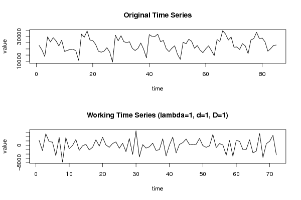
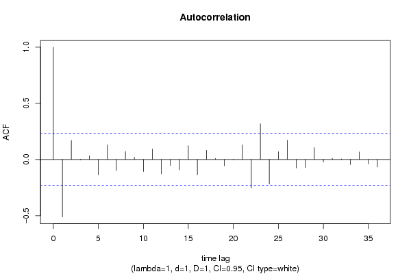
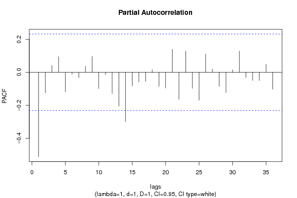
Title produced by software

(Partial) Autocorrelation Function

Date of computation

Fri, 02 Dec 2011 12:27:15 -0500

Cite this page as follows

Statistical Computations at FreeStatistics.org, Office for Research Development and Education, URL https://freestatistics.org/blog/index.php?v=date/2011/Dec/02/t1322846852rl979nn4ur640rl.htm/, Retrieved Mon, 29 Apr 2024 07:17:46 +0000

Statistical Computations at FreeStatistics.org, Office for Research Development and Education, URL https://freestatistics.org/blog/index.php?pk=150326, Retrieved Mon, 29 Apr 2024 07:17:46 +0000

QR Codes:

Paste this QR Code to cite your computation.

Original text written by user:

IsPrivate?

No (this computation is public)

User-defined keywords

Estimated Impact

120

Family? (F = Feedback message, R = changed R code, M = changed R Module, P = changed Parameters, D = changed Data)

-     [Univariate Explorative Data Analysis] [Run Sequence gebo...] [2008-12-12 13:32:37] [76963dc1903f0f612b6153510a3818cf]
- R  D  [Univariate Explorative Data Analysis] [Run Sequence gebo...] [2008-12-17 12:14:40] [76963dc1903f0f612b6153510a3818cf]
-         [Univariate Explorative Data Analysis] [Run Sequence Plot...] [2008-12-22 18:19:51] [1ce0d16c8f4225c977b42c8fa93bc163]
- RMP       [(Partial) Autocorrelation Function] [Identifying Integ...] [2009-11-22 12:16:10] [b98453cac15ba1066b407e146608df68]
-    D        [(Partial) Autocorrelation Function] [ACF van Y(t) (d=0...] [2009-11-26 00:58:58] [9717cb857c153ca3061376906953b329]
- R PD            [(Partial) Autocorrelation Function] [WS 9 ACF] [2011-12-02 17:27:15] [c98b04636162cea751932dfe577607eb] [Current]

Feedback Forum

Post a new message

Dataseries X:

Download CSV

Histogram

Boxplots

Summary of computational transaction
Raw Input	view raw input (R code)
Raw Output	view raw output of R engine
Computing time	1 seconds
R Server	'Gwilym Jenkins' @ jenkins.wessa.net

\begin{tabular}{lllllllll}
\hline
Summary of computational transaction \tabularnewline
Raw Input & view raw input (R code)  \tabularnewline
Raw Output & view raw output of R engine  \tabularnewline
Computing time & 1 seconds \tabularnewline
R Server & 'Gwilym Jenkins' @ jenkins.wessa.net \tabularnewline
\hline
\end{tabular}
%Source: https://freestatistics.org/blog/index.php?pk=150326&T=0

[TABLE]
[ROW][C]Summary of computational transaction[/C][/ROW]
[ROW][C]Raw Input[/C][C]view raw input (R code) [/C][/ROW]
[ROW][C]Raw Output[/C][C]view raw output of R engine [/C][/ROW]
[ROW][C]Computing time[/C][C]1 seconds[/C][/ROW]
[ROW][C]R Server[/C][C]'Gwilym Jenkins' @ jenkins.wessa.net[/C][/ROW]
[/TABLE]
Source: https://freestatistics.org/blog/index.php?pk=150326&T=0

Globally Unique Identifier (entire table): ba.freestatistics.org/blog/index.php?pk=150326&T=0

As an alternative you can also use a QR Code:

The GUIDs for individual cells are displayed in the table below:

Summary of computational transaction
Raw Input	view raw input (R code)
Raw Output	view raw output of R engine
Computing time	1 seconds
R Server	'Gwilym Jenkins' @ jenkins.wessa.net

Autocorrelation Function
Time lag k	ACF(k)	T-STAT	P-value
1	-0.511373	-4.3391	2.3e-05
2	0.169494	1.4382	0.077354
3	-0.004437	-0.0376	0.485037
4	0.033185	0.2816	0.389536
5	-0.136102	-1.1549	0.125983
6	0.130149	1.1043	0.13656
7	-0.097896	-0.8307	0.204451
8	0.071307	0.6051	0.273521
9	0.019396	0.1646	0.434867
10	-0.107112	-0.9089	0.183225
11	0.093947	0.7972	0.213989
12	-0.128623	-1.0914	0.139367
13	-0.052859	-0.4485	0.32756
14	-0.093042	-0.7895	0.216211
15	0.122966	1.0434	0.150127
16	-0.135557	-1.1502	0.126926
17	0.081024	0.6875	0.246985
18	0.008888	0.0754	0.470047
19	-0.056437	-0.4789	0.316735
20	-0.004556	-0.0387	0.484635
21	0.13065	1.1086	0.135647
22	-0.254789	-2.162	0.016973
23	0.317574	2.6947	0.004381
24	-0.219391	-1.8616	0.033371
25	0.069337	0.5883	0.279072
26	0.171387	1.4543	0.075109
27	-0.07486	-0.6352	0.263652
28	-0.071187	-0.604	0.273856
29	0.105778	0.8976	0.186208
30	-0.022869	-0.1941	0.42334
31	0.010492	0.089	0.464652
32	0.005449	0.0462	0.481626
33	-0.045474	-0.3859	0.35037
34	0.067155	0.5698	0.285285
35	-0.039519	-0.3353	0.369176
36	-0.067485	-0.5726	0.28434

\begin{tabular}{lllllllll}
\hline
Autocorrelation Function \tabularnewline
Time lag k & ACF(k) & T-STAT & P-value \tabularnewline
1 & -0.511373 & -4.3391 & 2.3e-05 \tabularnewline
2 & 0.169494 & 1.4382 & 0.077354 \tabularnewline
3 & -0.004437 & -0.0376 & 0.485037 \tabularnewline
4 & 0.033185 & 0.2816 & 0.389536 \tabularnewline
5 & -0.136102 & -1.1549 & 0.125983 \tabularnewline
6 & 0.130149 & 1.1043 & 0.13656 \tabularnewline
7 & -0.097896 & -0.8307 & 0.204451 \tabularnewline
8 & 0.071307 & 0.6051 & 0.273521 \tabularnewline
9 & 0.019396 & 0.1646 & 0.434867 \tabularnewline
10 & -0.107112 & -0.9089 & 0.183225 \tabularnewline
11 & 0.093947 & 0.7972 & 0.213989 \tabularnewline
12 & -0.128623 & -1.0914 & 0.139367 \tabularnewline
13 & -0.052859 & -0.4485 & 0.32756 \tabularnewline
14 & -0.093042 & -0.7895 & 0.216211 \tabularnewline
15 & 0.122966 & 1.0434 & 0.150127 \tabularnewline
16 & -0.135557 & -1.1502 & 0.126926 \tabularnewline
17 & 0.081024 & 0.6875 & 0.246985 \tabularnewline
18 & 0.008888 & 0.0754 & 0.470047 \tabularnewline
19 & -0.056437 & -0.4789 & 0.316735 \tabularnewline
20 & -0.004556 & -0.0387 & 0.484635 \tabularnewline
21 & 0.13065 & 1.1086 & 0.135647 \tabularnewline
22 & -0.254789 & -2.162 & 0.016973 \tabularnewline
23 & 0.317574 & 2.6947 & 0.004381 \tabularnewline
24 & -0.219391 & -1.8616 & 0.033371 \tabularnewline
25 & 0.069337 & 0.5883 & 0.279072 \tabularnewline
26 & 0.171387 & 1.4543 & 0.075109 \tabularnewline
27 & -0.07486 & -0.6352 & 0.263652 \tabularnewline
28 & -0.071187 & -0.604 & 0.273856 \tabularnewline
29 & 0.105778 & 0.8976 & 0.186208 \tabularnewline
30 & -0.022869 & -0.1941 & 0.42334 \tabularnewline
31 & 0.010492 & 0.089 & 0.464652 \tabularnewline
32 & 0.005449 & 0.0462 & 0.481626 \tabularnewline
33 & -0.045474 & -0.3859 & 0.35037 \tabularnewline
34 & 0.067155 & 0.5698 & 0.285285 \tabularnewline
35 & -0.039519 & -0.3353 & 0.369176 \tabularnewline
36 & -0.067485 & -0.5726 & 0.28434 \tabularnewline
\hline
\end{tabular}
%Source: https://freestatistics.org/blog/index.php?pk=150326&T=1

[TABLE]
[ROW][C]Autocorrelation Function[/C][/ROW]
[ROW][C]Time lag k[/C][C]ACF(k)[/C][C]T-STAT[/C][C]P-value[/C][/ROW]
[ROW][C]1[/C][C]-0.511373[/C][C]-4.3391[/C][C]2.3e-05[/C][/ROW]
[ROW][C]2[/C][C]0.169494[/C][C]1.4382[/C][C]0.077354[/C][/ROW]
[ROW][C]3[/C][C]-0.004437[/C][C]-0.0376[/C][C]0.485037[/C][/ROW]
[ROW][C]4[/C][C]0.033185[/C][C]0.2816[/C][C]0.389536[/C][/ROW]
[ROW][C]5[/C][C]-0.136102[/C][C]-1.1549[/C][C]0.125983[/C][/ROW]
[ROW][C]6[/C][C]0.130149[/C][C]1.1043[/C][C]0.13656[/C][/ROW]
[ROW][C]7[/C][C]-0.097896[/C][C]-0.8307[/C][C]0.204451[/C][/ROW]
[ROW][C]8[/C][C]0.071307[/C][C]0.6051[/C][C]0.273521[/C][/ROW]
[ROW][C]9[/C][C]0.019396[/C][C]0.1646[/C][C]0.434867[/C][/ROW]
[ROW][C]10[/C][C]-0.107112[/C][C]-0.9089[/C][C]0.183225[/C][/ROW]
[ROW][C]11[/C][C]0.093947[/C][C]0.7972[/C][C]0.213989[/C][/ROW]
[ROW][C]12[/C][C]-0.128623[/C][C]-1.0914[/C][C]0.139367[/C][/ROW]
[ROW][C]13[/C][C]-0.052859[/C][C]-0.4485[/C][C]0.32756[/C][/ROW]
[ROW][C]14[/C][C]-0.093042[/C][C]-0.7895[/C][C]0.216211[/C][/ROW]
[ROW][C]15[/C][C]0.122966[/C][C]1.0434[/C][C]0.150127[/C][/ROW]
[ROW][C]16[/C][C]-0.135557[/C][C]-1.1502[/C][C]0.126926[/C][/ROW]
[ROW][C]17[/C][C]0.081024[/C][C]0.6875[/C][C]0.246985[/C][/ROW]
[ROW][C]18[/C][C]0.008888[/C][C]0.0754[/C][C]0.470047[/C][/ROW]
[ROW][C]19[/C][C]-0.056437[/C][C]-0.4789[/C][C]0.316735[/C][/ROW]
[ROW][C]20[/C][C]-0.004556[/C][C]-0.0387[/C][C]0.484635[/C][/ROW]
[ROW][C]21[/C][C]0.13065[/C][C]1.1086[/C][C]0.135647[/C][/ROW]
[ROW][C]22[/C][C]-0.254789[/C][C]-2.162[/C][C]0.016973[/C][/ROW]
[ROW][C]23[/C][C]0.317574[/C][C]2.6947[/C][C]0.004381[/C][/ROW]
[ROW][C]24[/C][C]-0.219391[/C][C]-1.8616[/C][C]0.033371[/C][/ROW]
[ROW][C]25[/C][C]0.069337[/C][C]0.5883[/C][C]0.279072[/C][/ROW]
[ROW][C]26[/C][C]0.171387[/C][C]1.4543[/C][C]0.075109[/C][/ROW]
[ROW][C]27[/C][C]-0.07486[/C][C]-0.6352[/C][C]0.263652[/C][/ROW]
[ROW][C]28[/C][C]-0.071187[/C][C]-0.604[/C][C]0.273856[/C][/ROW]
[ROW][C]29[/C][C]0.105778[/C][C]0.8976[/C][C]0.186208[/C][/ROW]
[ROW][C]30[/C][C]-0.022869[/C][C]-0.1941[/C][C]0.42334[/C][/ROW]
[ROW][C]31[/C][C]0.010492[/C][C]0.089[/C][C]0.464652[/C][/ROW]
[ROW][C]32[/C][C]0.005449[/C][C]0.0462[/C][C]0.481626[/C][/ROW]
[ROW][C]33[/C][C]-0.045474[/C][C]-0.3859[/C][C]0.35037[/C][/ROW]
[ROW][C]34[/C][C]0.067155[/C][C]0.5698[/C][C]0.285285[/C][/ROW]
[ROW][C]35[/C][C]-0.039519[/C][C]-0.3353[/C][C]0.369176[/C][/ROW]
[ROW][C]36[/C][C]-0.067485[/C][C]-0.5726[/C][C]0.28434[/C][/ROW]
[/TABLE]
Source: https://freestatistics.org/blog/index.php?pk=150326&T=1

Globally Unique Identifier (entire table): ba.freestatistics.org/blog/index.php?pk=150326&T=1

As an alternative you can also use a QR Code:

The GUIDs for individual cells are displayed in the table below:

Autocorrelation Function
Time lag k	ACF(k)	T-STAT	P-value
1	-0.511373	-4.3391	2.3e-05
2	0.169494	1.4382	0.077354
3	-0.004437	-0.0376	0.485037
4	0.033185	0.2816	0.389536
5	-0.136102	-1.1549	0.125983
6	0.130149	1.1043	0.13656
7	-0.097896	-0.8307	0.204451
8	0.071307	0.6051	0.273521
9	0.019396	0.1646	0.434867
10	-0.107112	-0.9089	0.183225
11	0.093947	0.7972	0.213989
12	-0.128623	-1.0914	0.139367
13	-0.052859	-0.4485	0.32756
14	-0.093042	-0.7895	0.216211
15	0.122966	1.0434	0.150127
16	-0.135557	-1.1502	0.126926
17	0.081024	0.6875	0.246985
18	0.008888	0.0754	0.470047
19	-0.056437	-0.4789	0.316735
20	-0.004556	-0.0387	0.484635
21	0.13065	1.1086	0.135647
22	-0.254789	-2.162	0.016973
23	0.317574	2.6947	0.004381
24	-0.219391	-1.8616	0.033371
25	0.069337	0.5883	0.279072
26	0.171387	1.4543	0.075109
27	-0.07486	-0.6352	0.263652
28	-0.071187	-0.604	0.273856
29	0.105778	0.8976	0.186208
30	-0.022869	-0.1941	0.42334
31	0.010492	0.089	0.464652
32	0.005449	0.0462	0.481626
33	-0.045474	-0.3859	0.35037
34	0.067155	0.5698	0.285285
35	-0.039519	-0.3353	0.369176
36	-0.067485	-0.5726	0.28434

Partial Autocorrelation Function
Time lag k	PACF(k)	T-STAT	P-value
1	-0.511373	-4.3391	2.3e-05
2	-0.124588	-1.0572	0.146985
3	0.040336	0.3423	0.366575
4	0.094327	0.8004	0.213058
5	-0.118405	-1.0047	0.159202
6	-0.011855	-0.1006	0.460077
7	-0.032379	-0.2747	0.392151
8	0.036213	0.3073	0.37976
9	0.096375	0.8178	0.208093
10	-0.099058	-0.8405	0.201696
11	-0.014204	-0.1205	0.4522
12	-0.128616	-1.0913	0.139381
13	-0.205445	-1.7433	0.042778
14	-0.298677	-2.5344	0.00672
15	-0.082502	-0.7	0.243076
16	-0.058974	-0.5004	0.309155
17	-0.055342	-0.4696	0.320031
18	0.015774	0.1338	0.446949
19	-0.085373	-0.7244	0.235579
20	-0.095414	-0.8096	0.210414
21	0.139014	1.1796	0.121027
22	-0.16492	-1.3994	0.082994
23	0.128607	1.0913	0.139397
24	-0.097512	-0.8274	0.205367
25	-0.16971	-1.44	0.077096
26	0.110888	0.9409	0.174947
27	0.020499	0.1739	0.431199
28	-0.086612	-0.7349	0.232384
29	-0.12242	-1.0388	0.151194
30	0.014934	0.1267	0.449759
31	0.128537	1.0907	0.139527
32	-0.03182	-0.27	0.393965
33	-0.049434	-0.4195	0.338063
34	-0.049647	-0.4213	0.337407
35	0.048266	0.4096	0.341675
36	-0.102702	-0.8715	0.193202

\begin{tabular}{lllllllll}
\hline
Partial Autocorrelation Function \tabularnewline
Time lag k & PACF(k) & T-STAT & P-value \tabularnewline
1 & -0.511373 & -4.3391 & 2.3e-05 \tabularnewline
2 & -0.124588 & -1.0572 & 0.146985 \tabularnewline
3 & 0.040336 & 0.3423 & 0.366575 \tabularnewline
4 & 0.094327 & 0.8004 & 0.213058 \tabularnewline
5 & -0.118405 & -1.0047 & 0.159202 \tabularnewline
6 & -0.011855 & -0.1006 & 0.460077 \tabularnewline
7 & -0.032379 & -0.2747 & 0.392151 \tabularnewline
8 & 0.036213 & 0.3073 & 0.37976 \tabularnewline
9 & 0.096375 & 0.8178 & 0.208093 \tabularnewline
10 & -0.099058 & -0.8405 & 0.201696 \tabularnewline
11 & -0.014204 & -0.1205 & 0.4522 \tabularnewline
12 & -0.128616 & -1.0913 & 0.139381 \tabularnewline
13 & -0.205445 & -1.7433 & 0.042778 \tabularnewline
14 & -0.298677 & -2.5344 & 0.00672 \tabularnewline
15 & -0.082502 & -0.7 & 0.243076 \tabularnewline
16 & -0.058974 & -0.5004 & 0.309155 \tabularnewline
17 & -0.055342 & -0.4696 & 0.320031 \tabularnewline
18 & 0.015774 & 0.1338 & 0.446949 \tabularnewline
19 & -0.085373 & -0.7244 & 0.235579 \tabularnewline
20 & -0.095414 & -0.8096 & 0.210414 \tabularnewline
21 & 0.139014 & 1.1796 & 0.121027 \tabularnewline
22 & -0.16492 & -1.3994 & 0.082994 \tabularnewline
23 & 0.128607 & 1.0913 & 0.139397 \tabularnewline
24 & -0.097512 & -0.8274 & 0.205367 \tabularnewline
25 & -0.16971 & -1.44 & 0.077096 \tabularnewline
26 & 0.110888 & 0.9409 & 0.174947 \tabularnewline
27 & 0.020499 & 0.1739 & 0.431199 \tabularnewline
28 & -0.086612 & -0.7349 & 0.232384 \tabularnewline
29 & -0.12242 & -1.0388 & 0.151194 \tabularnewline
30 & 0.014934 & 0.1267 & 0.449759 \tabularnewline
31 & 0.128537 & 1.0907 & 0.139527 \tabularnewline
32 & -0.03182 & -0.27 & 0.393965 \tabularnewline
33 & -0.049434 & -0.4195 & 0.338063 \tabularnewline
34 & -0.049647 & -0.4213 & 0.337407 \tabularnewline
35 & 0.048266 & 0.4096 & 0.341675 \tabularnewline
36 & -0.102702 & -0.8715 & 0.193202 \tabularnewline
\hline
\end{tabular}
%Source: https://freestatistics.org/blog/index.php?pk=150326&T=2

[TABLE]
[ROW][C]Partial Autocorrelation Function[/C][/ROW]
[ROW][C]Time lag k[/C][C]PACF(k)[/C][C]T-STAT[/C][C]P-value[/C][/ROW]
[ROW][C]1[/C][C]-0.511373[/C][C]-4.3391[/C][C]2.3e-05[/C][/ROW]
[ROW][C]2[/C][C]-0.124588[/C][C]-1.0572[/C][C]0.146985[/C][/ROW]
[ROW][C]3[/C][C]0.040336[/C][C]0.3423[/C][C]0.366575[/C][/ROW]
[ROW][C]4[/C][C]0.094327[/C][C]0.8004[/C][C]0.213058[/C][/ROW]
[ROW][C]5[/C][C]-0.118405[/C][C]-1.0047[/C][C]0.159202[/C][/ROW]
[ROW][C]6[/C][C]-0.011855[/C][C]-0.1006[/C][C]0.460077[/C][/ROW]
[ROW][C]7[/C][C]-0.032379[/C][C]-0.2747[/C][C]0.392151[/C][/ROW]
[ROW][C]8[/C][C]0.036213[/C][C]0.3073[/C][C]0.37976[/C][/ROW]
[ROW][C]9[/C][C]0.096375[/C][C]0.8178[/C][C]0.208093[/C][/ROW]
[ROW][C]10[/C][C]-0.099058[/C][C]-0.8405[/C][C]0.201696[/C][/ROW]
[ROW][C]11[/C][C]-0.014204[/C][C]-0.1205[/C][C]0.4522[/C][/ROW]
[ROW][C]12[/C][C]-0.128616[/C][C]-1.0913[/C][C]0.139381[/C][/ROW]
[ROW][C]13[/C][C]-0.205445[/C][C]-1.7433[/C][C]0.042778[/C][/ROW]
[ROW][C]14[/C][C]-0.298677[/C][C]-2.5344[/C][C]0.00672[/C][/ROW]
[ROW][C]15[/C][C]-0.082502[/C][C]-0.7[/C][C]0.243076[/C][/ROW]
[ROW][C]16[/C][C]-0.058974[/C][C]-0.5004[/C][C]0.309155[/C][/ROW]
[ROW][C]17[/C][C]-0.055342[/C][C]-0.4696[/C][C]0.320031[/C][/ROW]
[ROW][C]18[/C][C]0.015774[/C][C]0.1338[/C][C]0.446949[/C][/ROW]
[ROW][C]19[/C][C]-0.085373[/C][C]-0.7244[/C][C]0.235579[/C][/ROW]
[ROW][C]20[/C][C]-0.095414[/C][C]-0.8096[/C][C]0.210414[/C][/ROW]
[ROW][C]21[/C][C]0.139014[/C][C]1.1796[/C][C]0.121027[/C][/ROW]
[ROW][C]22[/C][C]-0.16492[/C][C]-1.3994[/C][C]0.082994[/C][/ROW]
[ROW][C]23[/C][C]0.128607[/C][C]1.0913[/C][C]0.139397[/C][/ROW]
[ROW][C]24[/C][C]-0.097512[/C][C]-0.8274[/C][C]0.205367[/C][/ROW]
[ROW][C]25[/C][C]-0.16971[/C][C]-1.44[/C][C]0.077096[/C][/ROW]
[ROW][C]26[/C][C]0.110888[/C][C]0.9409[/C][C]0.174947[/C][/ROW]
[ROW][C]27[/C][C]0.020499[/C][C]0.1739[/C][C]0.431199[/C][/ROW]
[ROW][C]28[/C][C]-0.086612[/C][C]-0.7349[/C][C]0.232384[/C][/ROW]
[ROW][C]29[/C][C]-0.12242[/C][C]-1.0388[/C][C]0.151194[/C][/ROW]
[ROW][C]30[/C][C]0.014934[/C][C]0.1267[/C][C]0.449759[/C][/ROW]
[ROW][C]31[/C][C]0.128537[/C][C]1.0907[/C][C]0.139527[/C][/ROW]
[ROW][C]32[/C][C]-0.03182[/C][C]-0.27[/C][C]0.393965[/C][/ROW]
[ROW][C]33[/C][C]-0.049434[/C][C]-0.4195[/C][C]0.338063[/C][/ROW]
[ROW][C]34[/C][C]-0.049647[/C][C]-0.4213[/C][C]0.337407[/C][/ROW]
[ROW][C]35[/C][C]0.048266[/C][C]0.4096[/C][C]0.341675[/C][/ROW]
[ROW][C]36[/C][C]-0.102702[/C][C]-0.8715[/C][C]0.193202[/C][/ROW]
[/TABLE]
Source: https://freestatistics.org/blog/index.php?pk=150326&T=2

Globally Unique Identifier (entire table): ba.freestatistics.org/blog/index.php?pk=150326&T=2

As an alternative you can also use a QR Code:

The GUIDs for individual cells are displayed in the table below:

Partial Autocorrelation Function
Time lag k	PACF(k)	T-STAT	P-value
1	-0.511373	-4.3391	2.3e-05
2	-0.124588	-1.0572	0.146985
3	0.040336	0.3423	0.366575
4	0.094327	0.8004	0.213058
5	-0.118405	-1.0047	0.159202
6	-0.011855	-0.1006	0.460077
7	-0.032379	-0.2747	0.392151
8	0.036213	0.3073	0.37976
9	0.096375	0.8178	0.208093
10	-0.099058	-0.8405	0.201696
11	-0.014204	-0.1205	0.4522
12	-0.128616	-1.0913	0.139381
13	-0.205445	-1.7433	0.042778
14	-0.298677	-2.5344	0.00672
15	-0.082502	-0.7	0.243076
16	-0.058974	-0.5004	0.309155
17	-0.055342	-0.4696	0.320031
18	0.015774	0.1338	0.446949
19	-0.085373	-0.7244	0.235579
20	-0.095414	-0.8096	0.210414
21	0.139014	1.1796	0.121027
22	-0.16492	-1.3994	0.082994
23	0.128607	1.0913	0.139397
24	-0.097512	-0.8274	0.205367
25	-0.16971	-1.44	0.077096
26	0.110888	0.9409	0.174947
27	0.020499	0.1739	0.431199
28	-0.086612	-0.7349	0.232384
29	-0.12242	-1.0388	0.151194
30	0.014934	0.1267	0.449759
31	0.128537	1.0907	0.139527
32	-0.03182	-0.27	0.393965
33	-0.049434	-0.4195	0.338063
34	-0.049647	-0.4213	0.337407
35	0.048266	0.4096	0.341675
36	-0.102702	-0.8715	0.193202

Figure 1

PNG link

Postscript link

PDF link

Figure 2

PNG link

Postscript link

PDF link

Figure 3

PNG link

Postscript link

PDF link

Parameters (Session):

par1 = 48 ; par2 = 1 ; par3 = 0 ; par4 = 0 ; par5 = 12 ; par6 = White Noise ; par7 = 0.95 ;

Parameters (R input):

par1 = 36 ; par2 = 1 ; par3 = 1 ; par4 = 1 ; par5 = 12 ; par6 = White Noise ; par7 = 0.95 ; par8 = ;

R code (references can be found in the software module):

if (par1 == 'Default') {
par1 = 10*log10(length(x))
} else {
par1 <- as.numeric(par1)
}
par2 <- as.numeric(par2)
par3 <- as.numeric(par3)
par4 <- as.numeric(par4)
par5 <- as.numeric(par5)
if (par6 == 'White Noise') par6 <- 'white' else par6 <- 'ma'
par7 <- as.numeric(par7)
if (par8 != '') par8 <- as.numeric(par8)
ox <- x
if (par8 == '') {
if (par2 == 0) {
x <- log(x)
} else {
x <- (x ^ par2 - 1) / par2
}
} else {
x <- log(x,base=par8)
}
if (par3 > 0) x <- diff(x,lag=1,difference=par3)
if (par4 > 0) x <- diff(x,lag=par5,difference=par4)
bitmap(file='picts.png')
op <- par(mfrow=c(2,1))
plot(ox,type='l',main='Original Time Series',xlab='time',ylab='value')
if (par8=='') {
mytitle <- paste('Working Time Series (lambda=',par2,', d=',par3,', D=',par4,')',sep='')
mysub <- paste('(lambda=',par2,', d=',par3,', D=',par4,', CI=', par7, ', CI type=',par6,')',sep='')
} else {
mytitle <- paste('Working Time Series (base=',par8,', d=',par3,', D=',par4,')',sep='')
mysub <- paste('(base=',par8,', d=',par3,', D=',par4,', CI=', par7, ', CI type=',par6,')',sep='')
}
plot(x,type='l', main=mytitle,xlab='time',ylab='value')
par(op)
dev.off()
bitmap(file='pic1.png')
racf <- acf(x, par1, main='Autocorrelation', xlab='time lag', ylab='ACF', ci.type=par6, ci=par7, sub=mysub)
dev.off()
bitmap(file='pic2.png')
rpacf <- pacf(x,par1,main='Partial Autocorrelation',xlab='lags',ylab='PACF',sub=mysub)
dev.off()
(myacf <- c(racf$acf))
(mypacf <- c(rpacf$acf))
lengthx <- length(x)
sqrtn <- sqrt(lengthx)
load(file='createtable')
a<-table.start()
a<-table.row.start(a)
a<-table.element(a,'Autocorrelation Function',4,TRUE)
a<-table.row.end(a)
a<-table.row.start(a)
a<-table.element(a,'Time lag k',header=TRUE)
a<-table.element(a,hyperlink('basics.htm','ACF(k)','click here for more information about the Autocorrelation Function'),header=TRUE)
a<-table.element(a,'T-STAT',header=TRUE)
a<-table.element(a,'P-value',header=TRUE)
a<-table.row.end(a)
for (i in 2:(par1+1)) {
a<-table.row.start(a)
a<-table.element(a,i-1,header=TRUE)
a<-table.element(a,round(myacf[i],6))
mytstat <- myacf[i]*sqrtn
a<-table.element(a,round(mytstat,4))
a<-table.element(a,round(1-pt(abs(mytstat),lengthx),6))
a<-table.row.end(a)
}
a<-table.end(a)
table.save(a,file='mytable.tab')
a<-table.start()
a<-table.row.start(a)
a<-table.element(a,'Partial Autocorrelation Function',4,TRUE)
a<-table.row.end(a)
a<-table.row.start(a)
a<-table.element(a,'Time lag k',header=TRUE)
a<-table.element(a,hyperlink('basics.htm','PACF(k)','click here for more information about the Partial Autocorrelation Function'),header=TRUE)
a<-table.element(a,'T-STAT',header=TRUE)
a<-table.element(a,'P-value',header=TRUE)
a<-table.row.end(a)
for (i in 1:par1) {
a<-table.row.start(a)
a<-table.element(a,i,header=TRUE)
a<-table.element(a,round(mypacf[i],6))
mytstat <- mypacf[i]*sqrtn
a<-table.element(a,round(mytstat,4))
a<-table.element(a,round(1-pt(abs(mytstat),lengthx),6))
a<-table.row.end(a)
}
a<-table.end(a)
table.save(a,file='mytable1.tab')

Free Statistics

Description of Statistical Computation

Tree of Dependent Computations

Dataset

Tables (Output of Computation)

Figures (Output of Computation)

Input Parameters & R Code