Repository of Reproducible Computations

Free Statistics

of Irreproducible Research!

Author's title

Author

*The author of this computation has been verified*

R Software Module

rwasp_autocorrelation.wasp

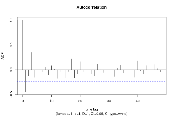
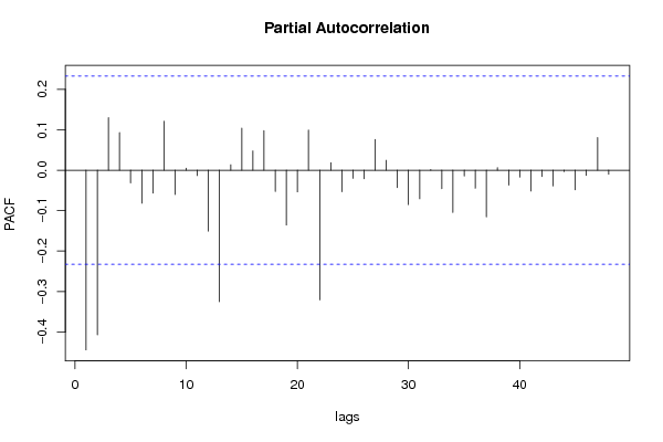
Title produced by software

(Partial) Autocorrelation Function

Date of computation

Fri, 02 Dec 2011 09:20:46 -0500

Cite this page as follows

Statistical Computations at FreeStatistics.org, Office for Research Development and Education, URL https://freestatistics.org/blog/index.php?v=date/2011/Dec/02/t1322835690dx3u9vvjmha2j8x.htm/, Retrieved Mon, 29 Apr 2024 03:18:26 +0000

Statistical Computations at FreeStatistics.org, Office for Research Development and Education, URL https://freestatistics.org/blog/index.php?pk=150237, Retrieved Mon, 29 Apr 2024 03:18:26 +0000

QR Codes:

Paste this QR Code to cite your computation.

Original text written by user:

IsPrivate?

No (this computation is public)

User-defined keywords

Estimated Impact

145

Family? (F = Feedback message, R = changed R code, M = changed R Module, P = changed Parameters, D = changed Data)

-     [Univariate Explorative Data Analysis] [Run Sequence gebo...] [2008-12-12 13:32:37] [76963dc1903f0f612b6153510a3818cf]
- R  D  [Univariate Explorative Data Analysis] [Run Sequence gebo...] [2008-12-17 12:14:40] [76963dc1903f0f612b6153510a3818cf]
-         [Univariate Explorative Data Analysis] [Run Sequence Plot...] [2008-12-22 18:19:51] [1ce0d16c8f4225c977b42c8fa93bc163]
- RMP       [Univariate Data Series] [Identifying Integ...] [2009-11-22 12:08:06] [b98453cac15ba1066b407e146608df68]
- RMP         [(Partial) Autocorrelation Function] [Births] [2010-11-29 09:36:27] [b98453cac15ba1066b407e146608df68]
- R PD          [(Partial) Autocorrelation Function] [WS9] [2011-12-02 13:40:33] [91ce4971c808115c699d50336245df56]
-   P               [(Partial) Autocorrelation Function] [WS9] [2011-12-02 14:20:46] [7a9891c1925ad1e8ddfe52b8c5887b5b] [Current]
- R P                 [(Partial) Autocorrelation Function] [] [2011-12-11 19:27:58] [84fecfa8c8107ac4e0024d8b1730a531] 

Feedback Forum

Post a new message

Dataseries X:

Download CSV

Histogram

Boxplots

Summary of computational transaction
Raw Input	view raw input (R code)
Raw Output	view raw output of R engine
Computing time	1 seconds
R Server	'Gertrude Mary Cox' @ cox.wessa.net

\begin{tabular}{lllllllll}
\hline
Summary of computational transaction \tabularnewline
Raw Input & view raw input (R code)  \tabularnewline
Raw Output & view raw output of R engine  \tabularnewline
Computing time & 1 seconds \tabularnewline
R Server & 'Gertrude Mary Cox' @ cox.wessa.net \tabularnewline
\hline
\end{tabular}
%Source: https://freestatistics.org/blog/index.php?pk=150237&T=0

[TABLE]
[ROW][C]Summary of computational transaction[/C][/ROW]
[ROW][C]Raw Input[/C][C]view raw input (R code) [/C][/ROW]
[ROW][C]Raw Output[/C][C]view raw output of R engine [/C][/ROW]
[ROW][C]Computing time[/C][C]1 seconds[/C][/ROW]
[ROW][C]R Server[/C][C]'Gertrude Mary Cox' @ cox.wessa.net[/C][/ROW]
[/TABLE]
Source: https://freestatistics.org/blog/index.php?pk=150237&T=0

Globally Unique Identifier (entire table): ba.freestatistics.org/blog/index.php?pk=150237&T=0

As an alternative you can also use a QR Code:

The GUIDs for individual cells are displayed in the table below:

Summary of computational transaction
Raw Input	view raw input (R code)
Raw Output	view raw output of R engine
Computing time	1 seconds
R Server	'Gertrude Mary Cox' @ cox.wessa.net

Autocorrelation Function
Time lag k	ACF(k)	T-STAT	P-value
1	-0.444343	-3.7441	0.000182
2	-0.129336	-1.0898	0.139742
3	0.348988	2.9406	0.002209
4	-0.15429	-1.3001	0.098891
5	-0.098522	-0.8302	0.204614
6	0.113972	0.9603	0.17007
7	-0.040085	-0.3378	0.368268
8	0.047524	0.4004	0.345017
9	-0.1024	-0.8628	0.195565
10	0.08317	0.7008	0.242858
11	0.009195	0.0775	0.469232
12	-0.173553	-1.4624	0.074024
13	-0.039054	-0.3291	0.371533
14	0.224607	1.8926	0.031246
15	-0.157937	-1.3308	0.093757
16	-0.035369	-0.298	0.383277
17	0.218812	1.8437	0.034697
18	-0.159004	-1.3398	0.092293
19	-0.079892	-0.6732	0.251508
20	0.163219	1.3753	0.08668
21	-0.043107	-0.3632	0.358759
22	-0.268125	-2.2593	0.013469
23	0.32916	2.7736	0.003539
24	-0.084802	-0.7146	0.238615
25	-0.118635	-0.9996	0.160441
26	0.113758	0.9585	0.170521
27	-0.002582	-0.0218	0.49135
28	-0.057018	-0.4804	0.316195
29	0.002841	0.0239	0.490484
30	-0.020964	-0.1766	0.430146
31	0.126065	1.0622	0.145863
32	-0.136331	-1.1487	0.127259
33	0.033772	0.2846	0.388403
34	0.099399	0.8376	0.202546
35	-0.066993	-0.5645	0.287099
36	-0.140026	-1.1799	0.120992
37	0.163421	1.377	0.086417
38	-0.024663	-0.2078	0.417984
39	-0.15369	-1.295	0.099756
40	0.180582	1.5216	0.066274
41	-0.021856	-0.1842	0.427204
42	-0.088183	-0.743	0.229953
43	0.084541	0.7124	0.23929
44	0.019082	0.1608	0.43636
45	-0.106133	-0.8943	0.187094
46	0.104733	0.8825	0.190243
47	0.023245	0.1959	0.422638
48	-0.043659	-0.3679	0.357031

\begin{tabular}{lllllllll}
\hline
Autocorrelation Function \tabularnewline
Time lag k & ACF(k) & T-STAT & P-value \tabularnewline
1 & -0.444343 & -3.7441 & 0.000182 \tabularnewline
2 & -0.129336 & -1.0898 & 0.139742 \tabularnewline
3 & 0.348988 & 2.9406 & 0.002209 \tabularnewline
4 & -0.15429 & -1.3001 & 0.098891 \tabularnewline
5 & -0.098522 & -0.8302 & 0.204614 \tabularnewline
6 & 0.113972 & 0.9603 & 0.17007 \tabularnewline
7 & -0.040085 & -0.3378 & 0.368268 \tabularnewline
8 & 0.047524 & 0.4004 & 0.345017 \tabularnewline
9 & -0.1024 & -0.8628 & 0.195565 \tabularnewline
10 & 0.08317 & 0.7008 & 0.242858 \tabularnewline
11 & 0.009195 & 0.0775 & 0.469232 \tabularnewline
12 & -0.173553 & -1.4624 & 0.074024 \tabularnewline
13 & -0.039054 & -0.3291 & 0.371533 \tabularnewline
14 & 0.224607 & 1.8926 & 0.031246 \tabularnewline
15 & -0.157937 & -1.3308 & 0.093757 \tabularnewline
16 & -0.035369 & -0.298 & 0.383277 \tabularnewline
17 & 0.218812 & 1.8437 & 0.034697 \tabularnewline
18 & -0.159004 & -1.3398 & 0.092293 \tabularnewline
19 & -0.079892 & -0.6732 & 0.251508 \tabularnewline
20 & 0.163219 & 1.3753 & 0.08668 \tabularnewline
21 & -0.043107 & -0.3632 & 0.358759 \tabularnewline
22 & -0.268125 & -2.2593 & 0.013469 \tabularnewline
23 & 0.32916 & 2.7736 & 0.003539 \tabularnewline
24 & -0.084802 & -0.7146 & 0.238615 \tabularnewline
25 & -0.118635 & -0.9996 & 0.160441 \tabularnewline
26 & 0.113758 & 0.9585 & 0.170521 \tabularnewline
27 & -0.002582 & -0.0218 & 0.49135 \tabularnewline
28 & -0.057018 & -0.4804 & 0.316195 \tabularnewline
29 & 0.002841 & 0.0239 & 0.490484 \tabularnewline
30 & -0.020964 & -0.1766 & 0.430146 \tabularnewline
31 & 0.126065 & 1.0622 & 0.145863 \tabularnewline
32 & -0.136331 & -1.1487 & 0.127259 \tabularnewline
33 & 0.033772 & 0.2846 & 0.388403 \tabularnewline
34 & 0.099399 & 0.8376 & 0.202546 \tabularnewline
35 & -0.066993 & -0.5645 & 0.287099 \tabularnewline
36 & -0.140026 & -1.1799 & 0.120992 \tabularnewline
37 & 0.163421 & 1.377 & 0.086417 \tabularnewline
38 & -0.024663 & -0.2078 & 0.417984 \tabularnewline
39 & -0.15369 & -1.295 & 0.099756 \tabularnewline
40 & 0.180582 & 1.5216 & 0.066274 \tabularnewline
41 & -0.021856 & -0.1842 & 0.427204 \tabularnewline
42 & -0.088183 & -0.743 & 0.229953 \tabularnewline
43 & 0.084541 & 0.7124 & 0.23929 \tabularnewline
44 & 0.019082 & 0.1608 & 0.43636 \tabularnewline
45 & -0.106133 & -0.8943 & 0.187094 \tabularnewline
46 & 0.104733 & 0.8825 & 0.190243 \tabularnewline
47 & 0.023245 & 0.1959 & 0.422638 \tabularnewline
48 & -0.043659 & -0.3679 & 0.357031 \tabularnewline
\hline
\end{tabular}
%Source: https://freestatistics.org/blog/index.php?pk=150237&T=1

[TABLE]
[ROW][C]Autocorrelation Function[/C][/ROW]
[ROW][C]Time lag k[/C][C]ACF(k)[/C][C]T-STAT[/C][C]P-value[/C][/ROW]
[ROW][C]1[/C][C]-0.444343[/C][C]-3.7441[/C][C]0.000182[/C][/ROW]
[ROW][C]2[/C][C]-0.129336[/C][C]-1.0898[/C][C]0.139742[/C][/ROW]
[ROW][C]3[/C][C]0.348988[/C][C]2.9406[/C][C]0.002209[/C][/ROW]
[ROW][C]4[/C][C]-0.15429[/C][C]-1.3001[/C][C]0.098891[/C][/ROW]
[ROW][C]5[/C][C]-0.098522[/C][C]-0.8302[/C][C]0.204614[/C][/ROW]
[ROW][C]6[/C][C]0.113972[/C][C]0.9603[/C][C]0.17007[/C][/ROW]
[ROW][C]7[/C][C]-0.040085[/C][C]-0.3378[/C][C]0.368268[/C][/ROW]
[ROW][C]8[/C][C]0.047524[/C][C]0.4004[/C][C]0.345017[/C][/ROW]
[ROW][C]9[/C][C]-0.1024[/C][C]-0.8628[/C][C]0.195565[/C][/ROW]
[ROW][C]10[/C][C]0.08317[/C][C]0.7008[/C][C]0.242858[/C][/ROW]
[ROW][C]11[/C][C]0.009195[/C][C]0.0775[/C][C]0.469232[/C][/ROW]
[ROW][C]12[/C][C]-0.173553[/C][C]-1.4624[/C][C]0.074024[/C][/ROW]
[ROW][C]13[/C][C]-0.039054[/C][C]-0.3291[/C][C]0.371533[/C][/ROW]
[ROW][C]14[/C][C]0.224607[/C][C]1.8926[/C][C]0.031246[/C][/ROW]
[ROW][C]15[/C][C]-0.157937[/C][C]-1.3308[/C][C]0.093757[/C][/ROW]
[ROW][C]16[/C][C]-0.035369[/C][C]-0.298[/C][C]0.383277[/C][/ROW]
[ROW][C]17[/C][C]0.218812[/C][C]1.8437[/C][C]0.034697[/C][/ROW]
[ROW][C]18[/C][C]-0.159004[/C][C]-1.3398[/C][C]0.092293[/C][/ROW]
[ROW][C]19[/C][C]-0.079892[/C][C]-0.6732[/C][C]0.251508[/C][/ROW]
[ROW][C]20[/C][C]0.163219[/C][C]1.3753[/C][C]0.08668[/C][/ROW]
[ROW][C]21[/C][C]-0.043107[/C][C]-0.3632[/C][C]0.358759[/C][/ROW]
[ROW][C]22[/C][C]-0.268125[/C][C]-2.2593[/C][C]0.013469[/C][/ROW]
[ROW][C]23[/C][C]0.32916[/C][C]2.7736[/C][C]0.003539[/C][/ROW]
[ROW][C]24[/C][C]-0.084802[/C][C]-0.7146[/C][C]0.238615[/C][/ROW]
[ROW][C]25[/C][C]-0.118635[/C][C]-0.9996[/C][C]0.160441[/C][/ROW]
[ROW][C]26[/C][C]0.113758[/C][C]0.9585[/C][C]0.170521[/C][/ROW]
[ROW][C]27[/C][C]-0.002582[/C][C]-0.0218[/C][C]0.49135[/C][/ROW]
[ROW][C]28[/C][C]-0.057018[/C][C]-0.4804[/C][C]0.316195[/C][/ROW]
[ROW][C]29[/C][C]0.002841[/C][C]0.0239[/C][C]0.490484[/C][/ROW]
[ROW][C]30[/C][C]-0.020964[/C][C]-0.1766[/C][C]0.430146[/C][/ROW]
[ROW][C]31[/C][C]0.126065[/C][C]1.0622[/C][C]0.145863[/C][/ROW]
[ROW][C]32[/C][C]-0.136331[/C][C]-1.1487[/C][C]0.127259[/C][/ROW]
[ROW][C]33[/C][C]0.033772[/C][C]0.2846[/C][C]0.388403[/C][/ROW]
[ROW][C]34[/C][C]0.099399[/C][C]0.8376[/C][C]0.202546[/C][/ROW]
[ROW][C]35[/C][C]-0.066993[/C][C]-0.5645[/C][C]0.287099[/C][/ROW]
[ROW][C]36[/C][C]-0.140026[/C][C]-1.1799[/C][C]0.120992[/C][/ROW]
[ROW][C]37[/C][C]0.163421[/C][C]1.377[/C][C]0.086417[/C][/ROW]
[ROW][C]38[/C][C]-0.024663[/C][C]-0.2078[/C][C]0.417984[/C][/ROW]
[ROW][C]39[/C][C]-0.15369[/C][C]-1.295[/C][C]0.099756[/C][/ROW]
[ROW][C]40[/C][C]0.180582[/C][C]1.5216[/C][C]0.066274[/C][/ROW]
[ROW][C]41[/C][C]-0.021856[/C][C]-0.1842[/C][C]0.427204[/C][/ROW]
[ROW][C]42[/C][C]-0.088183[/C][C]-0.743[/C][C]0.229953[/C][/ROW]
[ROW][C]43[/C][C]0.084541[/C][C]0.7124[/C][C]0.23929[/C][/ROW]
[ROW][C]44[/C][C]0.019082[/C][C]0.1608[/C][C]0.43636[/C][/ROW]
[ROW][C]45[/C][C]-0.106133[/C][C]-0.8943[/C][C]0.187094[/C][/ROW]
[ROW][C]46[/C][C]0.104733[/C][C]0.8825[/C][C]0.190243[/C][/ROW]
[ROW][C]47[/C][C]0.023245[/C][C]0.1959[/C][C]0.422638[/C][/ROW]
[ROW][C]48[/C][C]-0.043659[/C][C]-0.3679[/C][C]0.357031[/C][/ROW]
[/TABLE]
Source: https://freestatistics.org/blog/index.php?pk=150237&T=1

Globally Unique Identifier (entire table): ba.freestatistics.org/blog/index.php?pk=150237&T=1

As an alternative you can also use a QR Code:

The GUIDs for individual cells are displayed in the table below:

Autocorrelation Function
Time lag k	ACF(k)	T-STAT	P-value
1	-0.444343	-3.7441	0.000182
2	-0.129336	-1.0898	0.139742
3	0.348988	2.9406	0.002209
4	-0.15429	-1.3001	0.098891
5	-0.098522	-0.8302	0.204614
6	0.113972	0.9603	0.17007
7	-0.040085	-0.3378	0.368268
8	0.047524	0.4004	0.345017
9	-0.1024	-0.8628	0.195565
10	0.08317	0.7008	0.242858
11	0.009195	0.0775	0.469232
12	-0.173553	-1.4624	0.074024
13	-0.039054	-0.3291	0.371533
14	0.224607	1.8926	0.031246
15	-0.157937	-1.3308	0.093757
16	-0.035369	-0.298	0.383277
17	0.218812	1.8437	0.034697
18	-0.159004	-1.3398	0.092293
19	-0.079892	-0.6732	0.251508
20	0.163219	1.3753	0.08668
21	-0.043107	-0.3632	0.358759
22	-0.268125	-2.2593	0.013469
23	0.32916	2.7736	0.003539
24	-0.084802	-0.7146	0.238615
25	-0.118635	-0.9996	0.160441
26	0.113758	0.9585	0.170521
27	-0.002582	-0.0218	0.49135
28	-0.057018	-0.4804	0.316195
29	0.002841	0.0239	0.490484
30	-0.020964	-0.1766	0.430146
31	0.126065	1.0622	0.145863
32	-0.136331	-1.1487	0.127259
33	0.033772	0.2846	0.388403
34	0.099399	0.8376	0.202546
35	-0.066993	-0.5645	0.287099
36	-0.140026	-1.1799	0.120992
37	0.163421	1.377	0.086417
38	-0.024663	-0.2078	0.417984
39	-0.15369	-1.295	0.099756
40	0.180582	1.5216	0.066274
41	-0.021856	-0.1842	0.427204
42	-0.088183	-0.743	0.229953
43	0.084541	0.7124	0.23929
44	0.019082	0.1608	0.43636
45	-0.106133	-0.8943	0.187094
46	0.104733	0.8825	0.190243
47	0.023245	0.1959	0.422638
48	-0.043659	-0.3679	0.357031

Partial Autocorrelation Function
Time lag k	PACF(k)	T-STAT	P-value
1	-0.444343	-3.7441	0.000182
2	-0.407169	-3.4309	0.000503
3	0.130239	1.0974	0.138085
4	0.09292	0.783	0.218127
5	-0.031504	-0.2655	0.395714
6	-0.081506	-0.6868	0.247229
7	-0.05653	-0.4763	0.31765
8	0.121301	1.0221	0.155101
9	-0.05999	-0.5055	0.307392
10	0.005151	0.0434	0.482752
11	-0.013207	-0.1113	0.455853
12	-0.150437	-1.2676	0.104541
13	-0.324884	-2.7375	0.003909
14	0.01349	0.1137	0.454911
15	0.103847	0.875	0.192254
16	0.047765	0.4025	0.344273
17	0.097943	0.8253	0.205987
18	-0.052303	-0.4407	0.330381
19	-0.135502	-1.1418	0.128695
20	-0.053455	-0.4504	0.32689
21	0.099407	0.8376	0.202529
22	-0.32065	-2.7018	0.004309
23	0.018669	0.1573	0.437724
24	-0.053017	-0.4467	0.328217
25	-0.019985	-0.1684	0.433374
26	-0.021205	-0.1787	0.429349
27	0.076131	0.6415	0.261635
28	0.024459	0.2061	0.418654
29	-0.042699	-0.3598	0.360037
30	-0.084848	-0.7149	0.238494
31	-0.070581	-0.5947	0.276959
32	0.001807	0.0152	0.493947
33	-0.045475	-0.3832	0.351365
34	-0.104487	-0.8804	0.190801
35	-0.014387	-0.1212	0.451928
36	-0.044515	-0.3751	0.354356
37	-0.115119	-0.97	0.167666
38	0.006307	0.0531	0.478883
39	-0.036706	-0.3093	0.379003
40	-0.01679	-0.1415	0.443949
41	-0.051431	-0.4334	0.333032
42	-0.015705	-0.1323	0.447547
43	-0.039008	-0.3287	0.371681
44	-0.003369	-0.0284	0.488715
45	-0.048241	-0.4065	0.342804
46	-0.012715	-0.1071	0.457492
47	0.080966	0.6822	0.248655
48	-0.009835	-0.0829	0.467094

\begin{tabular}{lllllllll}
\hline
Partial Autocorrelation Function \tabularnewline
Time lag k & PACF(k) & T-STAT & P-value \tabularnewline
1 & -0.444343 & -3.7441 & 0.000182 \tabularnewline
2 & -0.407169 & -3.4309 & 0.000503 \tabularnewline
3 & 0.130239 & 1.0974 & 0.138085 \tabularnewline
4 & 0.09292 & 0.783 & 0.218127 \tabularnewline
5 & -0.031504 & -0.2655 & 0.395714 \tabularnewline
6 & -0.081506 & -0.6868 & 0.247229 \tabularnewline
7 & -0.05653 & -0.4763 & 0.31765 \tabularnewline
8 & 0.121301 & 1.0221 & 0.155101 \tabularnewline
9 & -0.05999 & -0.5055 & 0.307392 \tabularnewline
10 & 0.005151 & 0.0434 & 0.482752 \tabularnewline
11 & -0.013207 & -0.1113 & 0.455853 \tabularnewline
12 & -0.150437 & -1.2676 & 0.104541 \tabularnewline
13 & -0.324884 & -2.7375 & 0.003909 \tabularnewline
14 & 0.01349 & 0.1137 & 0.454911 \tabularnewline
15 & 0.103847 & 0.875 & 0.192254 \tabularnewline
16 & 0.047765 & 0.4025 & 0.344273 \tabularnewline
17 & 0.097943 & 0.8253 & 0.205987 \tabularnewline
18 & -0.052303 & -0.4407 & 0.330381 \tabularnewline
19 & -0.135502 & -1.1418 & 0.128695 \tabularnewline
20 & -0.053455 & -0.4504 & 0.32689 \tabularnewline
21 & 0.099407 & 0.8376 & 0.202529 \tabularnewline
22 & -0.32065 & -2.7018 & 0.004309 \tabularnewline
23 & 0.018669 & 0.1573 & 0.437724 \tabularnewline
24 & -0.053017 & -0.4467 & 0.328217 \tabularnewline
25 & -0.019985 & -0.1684 & 0.433374 \tabularnewline
26 & -0.021205 & -0.1787 & 0.429349 \tabularnewline
27 & 0.076131 & 0.6415 & 0.261635 \tabularnewline
28 & 0.024459 & 0.2061 & 0.418654 \tabularnewline
29 & -0.042699 & -0.3598 & 0.360037 \tabularnewline
30 & -0.084848 & -0.7149 & 0.238494 \tabularnewline
31 & -0.070581 & -0.5947 & 0.276959 \tabularnewline
32 & 0.001807 & 0.0152 & 0.493947 \tabularnewline
33 & -0.045475 & -0.3832 & 0.351365 \tabularnewline
34 & -0.104487 & -0.8804 & 0.190801 \tabularnewline
35 & -0.014387 & -0.1212 & 0.451928 \tabularnewline
36 & -0.044515 & -0.3751 & 0.354356 \tabularnewline
37 & -0.115119 & -0.97 & 0.167666 \tabularnewline
38 & 0.006307 & 0.0531 & 0.478883 \tabularnewline
39 & -0.036706 & -0.3093 & 0.379003 \tabularnewline
40 & -0.01679 & -0.1415 & 0.443949 \tabularnewline
41 & -0.051431 & -0.4334 & 0.333032 \tabularnewline
42 & -0.015705 & -0.1323 & 0.447547 \tabularnewline
43 & -0.039008 & -0.3287 & 0.371681 \tabularnewline
44 & -0.003369 & -0.0284 & 0.488715 \tabularnewline
45 & -0.048241 & -0.4065 & 0.342804 \tabularnewline
46 & -0.012715 & -0.1071 & 0.457492 \tabularnewline
47 & 0.080966 & 0.6822 & 0.248655 \tabularnewline
48 & -0.009835 & -0.0829 & 0.467094 \tabularnewline
\hline
\end{tabular}
%Source: https://freestatistics.org/blog/index.php?pk=150237&T=2

[TABLE]
[ROW][C]Partial Autocorrelation Function[/C][/ROW]
[ROW][C]Time lag k[/C][C]PACF(k)[/C][C]T-STAT[/C][C]P-value[/C][/ROW]
[ROW][C]1[/C][C]-0.444343[/C][C]-3.7441[/C][C]0.000182[/C][/ROW]
[ROW][C]2[/C][C]-0.407169[/C][C]-3.4309[/C][C]0.000503[/C][/ROW]
[ROW][C]3[/C][C]0.130239[/C][C]1.0974[/C][C]0.138085[/C][/ROW]
[ROW][C]4[/C][C]0.09292[/C][C]0.783[/C][C]0.218127[/C][/ROW]
[ROW][C]5[/C][C]-0.031504[/C][C]-0.2655[/C][C]0.395714[/C][/ROW]
[ROW][C]6[/C][C]-0.081506[/C][C]-0.6868[/C][C]0.247229[/C][/ROW]
[ROW][C]7[/C][C]-0.05653[/C][C]-0.4763[/C][C]0.31765[/C][/ROW]
[ROW][C]8[/C][C]0.121301[/C][C]1.0221[/C][C]0.155101[/C][/ROW]
[ROW][C]9[/C][C]-0.05999[/C][C]-0.5055[/C][C]0.307392[/C][/ROW]
[ROW][C]10[/C][C]0.005151[/C][C]0.0434[/C][C]0.482752[/C][/ROW]
[ROW][C]11[/C][C]-0.013207[/C][C]-0.1113[/C][C]0.455853[/C][/ROW]
[ROW][C]12[/C][C]-0.150437[/C][C]-1.2676[/C][C]0.104541[/C][/ROW]
[ROW][C]13[/C][C]-0.324884[/C][C]-2.7375[/C][C]0.003909[/C][/ROW]
[ROW][C]14[/C][C]0.01349[/C][C]0.1137[/C][C]0.454911[/C][/ROW]
[ROW][C]15[/C][C]0.103847[/C][C]0.875[/C][C]0.192254[/C][/ROW]
[ROW][C]16[/C][C]0.047765[/C][C]0.4025[/C][C]0.344273[/C][/ROW]
[ROW][C]17[/C][C]0.097943[/C][C]0.8253[/C][C]0.205987[/C][/ROW]
[ROW][C]18[/C][C]-0.052303[/C][C]-0.4407[/C][C]0.330381[/C][/ROW]
[ROW][C]19[/C][C]-0.135502[/C][C]-1.1418[/C][C]0.128695[/C][/ROW]
[ROW][C]20[/C][C]-0.053455[/C][C]-0.4504[/C][C]0.32689[/C][/ROW]
[ROW][C]21[/C][C]0.099407[/C][C]0.8376[/C][C]0.202529[/C][/ROW]
[ROW][C]22[/C][C]-0.32065[/C][C]-2.7018[/C][C]0.004309[/C][/ROW]
[ROW][C]23[/C][C]0.018669[/C][C]0.1573[/C][C]0.437724[/C][/ROW]
[ROW][C]24[/C][C]-0.053017[/C][C]-0.4467[/C][C]0.328217[/C][/ROW]
[ROW][C]25[/C][C]-0.019985[/C][C]-0.1684[/C][C]0.433374[/C][/ROW]
[ROW][C]26[/C][C]-0.021205[/C][C]-0.1787[/C][C]0.429349[/C][/ROW]
[ROW][C]27[/C][C]0.076131[/C][C]0.6415[/C][C]0.261635[/C][/ROW]
[ROW][C]28[/C][C]0.024459[/C][C]0.2061[/C][C]0.418654[/C][/ROW]
[ROW][C]29[/C][C]-0.042699[/C][C]-0.3598[/C][C]0.360037[/C][/ROW]
[ROW][C]30[/C][C]-0.084848[/C][C]-0.7149[/C][C]0.238494[/C][/ROW]
[ROW][C]31[/C][C]-0.070581[/C][C]-0.5947[/C][C]0.276959[/C][/ROW]
[ROW][C]32[/C][C]0.001807[/C][C]0.0152[/C][C]0.493947[/C][/ROW]
[ROW][C]33[/C][C]-0.045475[/C][C]-0.3832[/C][C]0.351365[/C][/ROW]
[ROW][C]34[/C][C]-0.104487[/C][C]-0.8804[/C][C]0.190801[/C][/ROW]
[ROW][C]35[/C][C]-0.014387[/C][C]-0.1212[/C][C]0.451928[/C][/ROW]
[ROW][C]36[/C][C]-0.044515[/C][C]-0.3751[/C][C]0.354356[/C][/ROW]
[ROW][C]37[/C][C]-0.115119[/C][C]-0.97[/C][C]0.167666[/C][/ROW]
[ROW][C]38[/C][C]0.006307[/C][C]0.0531[/C][C]0.478883[/C][/ROW]
[ROW][C]39[/C][C]-0.036706[/C][C]-0.3093[/C][C]0.379003[/C][/ROW]
[ROW][C]40[/C][C]-0.01679[/C][C]-0.1415[/C][C]0.443949[/C][/ROW]
[ROW][C]41[/C][C]-0.051431[/C][C]-0.4334[/C][C]0.333032[/C][/ROW]
[ROW][C]42[/C][C]-0.015705[/C][C]-0.1323[/C][C]0.447547[/C][/ROW]
[ROW][C]43[/C][C]-0.039008[/C][C]-0.3287[/C][C]0.371681[/C][/ROW]
[ROW][C]44[/C][C]-0.003369[/C][C]-0.0284[/C][C]0.488715[/C][/ROW]
[ROW][C]45[/C][C]-0.048241[/C][C]-0.4065[/C][C]0.342804[/C][/ROW]
[ROW][C]46[/C][C]-0.012715[/C][C]-0.1071[/C][C]0.457492[/C][/ROW]
[ROW][C]47[/C][C]0.080966[/C][C]0.6822[/C][C]0.248655[/C][/ROW]
[ROW][C]48[/C][C]-0.009835[/C][C]-0.0829[/C][C]0.467094[/C][/ROW]
[/TABLE]
Source: https://freestatistics.org/blog/index.php?pk=150237&T=2

Globally Unique Identifier (entire table): ba.freestatistics.org/blog/index.php?pk=150237&T=2

As an alternative you can also use a QR Code:

The GUIDs for individual cells are displayed in the table below:

Partial Autocorrelation Function
Time lag k	PACF(k)	T-STAT	P-value
1	-0.444343	-3.7441	0.000182
2	-0.407169	-3.4309	0.000503
3	0.130239	1.0974	0.138085
4	0.09292	0.783	0.218127
5	-0.031504	-0.2655	0.395714
6	-0.081506	-0.6868	0.247229
7	-0.05653	-0.4763	0.31765
8	0.121301	1.0221	0.155101
9	-0.05999	-0.5055	0.307392
10	0.005151	0.0434	0.482752
11	-0.013207	-0.1113	0.455853
12	-0.150437	-1.2676	0.104541
13	-0.324884	-2.7375	0.003909
14	0.01349	0.1137	0.454911
15	0.103847	0.875	0.192254
16	0.047765	0.4025	0.344273
17	0.097943	0.8253	0.205987
18	-0.052303	-0.4407	0.330381
19	-0.135502	-1.1418	0.128695
20	-0.053455	-0.4504	0.32689
21	0.099407	0.8376	0.202529
22	-0.32065	-2.7018	0.004309
23	0.018669	0.1573	0.437724
24	-0.053017	-0.4467	0.328217
25	-0.019985	-0.1684	0.433374
26	-0.021205	-0.1787	0.429349
27	0.076131	0.6415	0.261635
28	0.024459	0.2061	0.418654
29	-0.042699	-0.3598	0.360037
30	-0.084848	-0.7149	0.238494
31	-0.070581	-0.5947	0.276959
32	0.001807	0.0152	0.493947
33	-0.045475	-0.3832	0.351365
34	-0.104487	-0.8804	0.190801
35	-0.014387	-0.1212	0.451928
36	-0.044515	-0.3751	0.354356
37	-0.115119	-0.97	0.167666
38	0.006307	0.0531	0.478883
39	-0.036706	-0.3093	0.379003
40	-0.01679	-0.1415	0.443949
41	-0.051431	-0.4334	0.333032
42	-0.015705	-0.1323	0.447547
43	-0.039008	-0.3287	0.371681
44	-0.003369	-0.0284	0.488715
45	-0.048241	-0.4065	0.342804
46	-0.012715	-0.1071	0.457492
47	0.080966	0.6822	0.248655
48	-0.009835	-0.0829	0.467094

Figure 1

PNG link

Postscript link

PDF link

Figure 2

PNG link

Postscript link

PDF link

Parameters (Session):

par1 = 48 ; par2 = 1 ; par3 = 1 ; par4 = 1 ; par5 = 12 ; par6 = White Noise ; par7 = 0.95 ;

Parameters (R input):

par1 = 48 ; par2 = 1 ; par3 = 1 ; par4 = 1 ; par5 = 12 ; par6 = White Noise ; par7 = 0.95 ; par8 = ;

R code (references can be found in the software module):

if (par1 == 'Default') {
par1 = 10*log10(length(x))
} else {
par1 <- as.numeric(par1)
}
par2 <- as.numeric(par2)
par3 <- as.numeric(par3)
par4 <- as.numeric(par4)
par5 <- as.numeric(par5)
if (par6 == 'White Noise') par6 <- 'white' else par6 <- 'ma'
par7 <- as.numeric(par7)
if (par2 == 0) {
x <- log(x)
} else {
x <- (x ^ par2 - 1) / par2
}
if (par3 > 0) x <- diff(x,lag=1,difference=par3)
if (par4 > 0) x <- diff(x,lag=par5,difference=par4)
bitmap(file='pic1.png')
racf <- acf(x, par1, main='Autocorrelation', xlab='time lag', ylab='ACF', ci.type=par6, ci=par7, sub=paste('(lambda=',par2,', d=',par3,', D=',par4,', CI=', par7, ', CI type=',par6,')',sep=''))
dev.off()
bitmap(file='pic2.png')
rpacf <- pacf(x,par1,main='Partial Autocorrelation',xlab='lags',ylab='PACF')
dev.off()
(myacf <- c(racf$acf))
(mypacf <- c(rpacf$acf))
lengthx <- length(x)
sqrtn <- sqrt(lengthx)
load(file='createtable')
a<-table.start()
a<-table.row.start(a)
a<-table.element(a,'Autocorrelation Function',4,TRUE)
a<-table.row.end(a)
a<-table.row.start(a)
a<-table.element(a,'Time lag k',header=TRUE)
a<-table.element(a,hyperlink('basics.htm','ACF(k)','click here for more information about the Autocorrelation Function'),header=TRUE)
a<-table.element(a,'T-STAT',header=TRUE)
a<-table.element(a,'P-value',header=TRUE)
a<-table.row.end(a)
for (i in 2:(par1+1)) {
a<-table.row.start(a)
a<-table.element(a,i-1,header=TRUE)
a<-table.element(a,round(myacf[i],6))
mytstat <- myacf[i]*sqrtn
a<-table.element(a,round(mytstat,4))
a<-table.element(a,round(1-pt(abs(mytstat),lengthx),6))
a<-table.row.end(a)
}
a<-table.end(a)
table.save(a,file='mytable.tab')
a<-table.start()
a<-table.row.start(a)
a<-table.element(a,'Partial Autocorrelation Function',4,TRUE)
a<-table.row.end(a)
a<-table.row.start(a)
a<-table.element(a,'Time lag k',header=TRUE)
a<-table.element(a,hyperlink('basics.htm','PACF(k)','click here for more information about the Partial Autocorrelation Function'),header=TRUE)
a<-table.element(a,'T-STAT',header=TRUE)
a<-table.element(a,'P-value',header=TRUE)
a<-table.row.end(a)
for (i in 1:par1) {
a<-table.row.start(a)
a<-table.element(a,i,header=TRUE)
a<-table.element(a,round(mypacf[i],6))
mytstat <- mypacf[i]*sqrtn
a<-table.element(a,round(mytstat,4))
a<-table.element(a,round(1-pt(abs(mytstat),lengthx),6))
a<-table.row.end(a)
}
a<-table.end(a)
table.save(a,file='mytable1.tab')

Free Statistics

Description of Statistical Computation

Tree of Dependent Computations

Dataset

Tables (Output of Computation)

Figures (Output of Computation)

Input Parameters & R Code