Repository of Reproducible Computations

Free Statistics

of Irreproducible Research!

Author's title

Author

*The author of this computation has been verified*

R Software Module

rwasp_autocorrelation.wasp

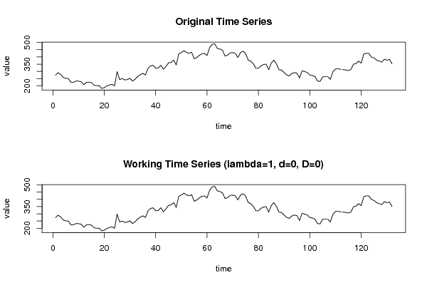
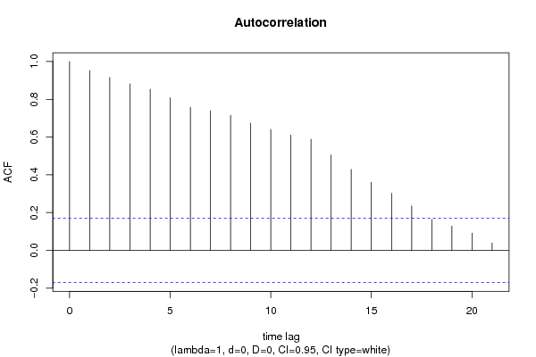
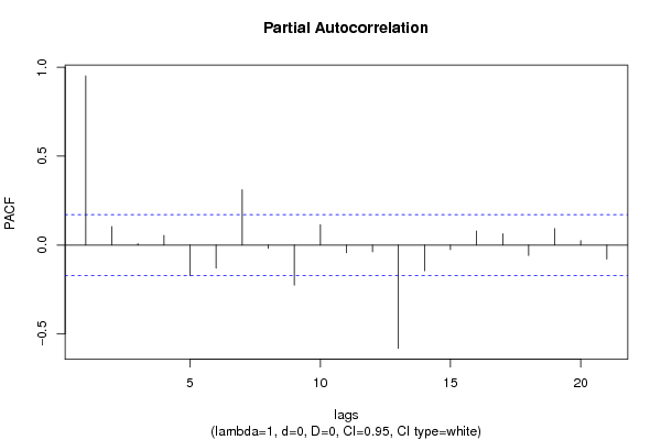
Title produced by software

(Partial) Autocorrelation Function

Date of computation

Thu, 01 Dec 2011 14:58:02 -0500

Cite this page as follows

Statistical Computations at FreeStatistics.org, Office for Research Development and Education, URL https://freestatistics.org/blog/index.php?v=date/2011/Dec/01/t13227695204trrrsbwaeoouvh.htm/, Retrieved Thu, 25 Apr 2024 22:43:03 +0000

Statistical Computations at FreeStatistics.org, Office for Research Development and Education, URL https://freestatistics.org/blog/index.php?pk=149978, Retrieved Thu, 25 Apr 2024 22:43:03 +0000

QR Codes:

Paste this QR Code to cite your computation.

Original text written by user:

IsPrivate?

No (this computation is public)

User-defined keywords

Estimated Impact

119

Family? (F = Feedback message, R = changed R code, M = changed R Module, P = changed Parameters, D = changed Data)

-       [(Partial) Autocorrelation Function] [] [2011-12-01 19:58:02] [7dc03dd48c8acabd98b217fada4a6bc0] [Current]
- R P     [(Partial) Autocorrelation Function] [] [2011-12-01 20:01:46] [ee8c3a74bf3b349877806e9a50913c60] 
-   P       [(Partial) Autocorrelation Function] [] [2011-12-01 20:04:38] [ee8c3a74bf3b349877806e9a50913c60] 
- RMP       [Spectral Analysis] [] [2011-12-01 20:13:31] [ee8c3a74bf3b349877806e9a50913c60] 
-   PD        [Spectral Analysis] [] [2011-12-01 21:22:24] [ee8c3a74bf3b349877806e9a50913c60] 
- RMP         [Standard Deviation-Mean Plot] [] [2011-12-01 21:39:37] [ee8c3a74bf3b349877806e9a50913c60] 
- R P         [Spectral Analysis] [verbetering] [2011-12-12 18:17:40] [25b6caf3839c2bdc14961e5bff2d6373] 

Feedback Forum

Post a new message

Dataseries X:

Download CSV

Histogram

Boxplots

Summary of computational transaction
Raw Input	view raw input (R code)
Raw Output	view raw output of R engine
Computing time	1 seconds
R Server	'Gertrude Mary Cox' @ cox.wessa.net

\begin{tabular}{lllllllll}
\hline
Summary of computational transaction \tabularnewline
Raw Input & view raw input (R code)  \tabularnewline
Raw Output & view raw output of R engine  \tabularnewline
Computing time & 1 seconds \tabularnewline
R Server & 'Gertrude Mary Cox' @ cox.wessa.net \tabularnewline
\hline
\end{tabular}
%Source: https://freestatistics.org/blog/index.php?pk=149978&T=0

[TABLE]
[ROW][C]Summary of computational transaction[/C][/ROW]
[ROW][C]Raw Input[/C][C]view raw input (R code) [/C][/ROW]
[ROW][C]Raw Output[/C][C]view raw output of R engine [/C][/ROW]
[ROW][C]Computing time[/C][C]1 seconds[/C][/ROW]
[ROW][C]R Server[/C][C]'Gertrude Mary Cox' @ cox.wessa.net[/C][/ROW]
[/TABLE]
Source: https://freestatistics.org/blog/index.php?pk=149978&T=0

Globally Unique Identifier (entire table): ba.freestatistics.org/blog/index.php?pk=149978&T=0

As an alternative you can also use a QR Code:

The GUIDs for individual cells are displayed in the table below:

Summary of computational transaction
Raw Input	view raw input (R code)
Raw Output	view raw output of R engine
Computing time	1 seconds
R Server	'Gertrude Mary Cox' @ cox.wessa.net

Autocorrelation Function
Time lag k	ACF(k)	T-STAT	P-value
1	0.952194	10.9399	0
2	0.916355	10.5281	0
3	0.881585	10.1286	0
4	0.853079	9.8011	0
5	0.808504	9.289	0
6	0.757877	8.7073	0
7	0.739452	8.4957	0
8	0.715406	8.2194	0
9	0.674109	7.7449	0
10	0.640434	7.358	0
11	0.611507	7.0257	0
12	0.588605	6.7626	0
13	0.505057	5.8027	0
14	0.429564	4.9353	1e-06
15	0.360785	4.1451	3e-05
16	0.302294	3.4731	0.000348
17	0.234717	2.6967	0.003958
18	0.16372	1.881	0.031088
19	0.128571	1.4772	0.071006
20	0.091046	1.046	0.148728
21	0.03893	0.4473	0.327707

\begin{tabular}{lllllllll}
\hline
Autocorrelation Function \tabularnewline
Time lag k & ACF(k) & T-STAT & P-value \tabularnewline
1 & 0.952194 & 10.9399 & 0 \tabularnewline
2 & 0.916355 & 10.5281 & 0 \tabularnewline
3 & 0.881585 & 10.1286 & 0 \tabularnewline
4 & 0.853079 & 9.8011 & 0 \tabularnewline
5 & 0.808504 & 9.289 & 0 \tabularnewline
6 & 0.757877 & 8.7073 & 0 \tabularnewline
7 & 0.739452 & 8.4957 & 0 \tabularnewline
8 & 0.715406 & 8.2194 & 0 \tabularnewline
9 & 0.674109 & 7.7449 & 0 \tabularnewline
10 & 0.640434 & 7.358 & 0 \tabularnewline
11 & 0.611507 & 7.0257 & 0 \tabularnewline
12 & 0.588605 & 6.7626 & 0 \tabularnewline
13 & 0.505057 & 5.8027 & 0 \tabularnewline
14 & 0.429564 & 4.9353 & 1e-06 \tabularnewline
15 & 0.360785 & 4.1451 & 3e-05 \tabularnewline
16 & 0.302294 & 3.4731 & 0.000348 \tabularnewline
17 & 0.234717 & 2.6967 & 0.003958 \tabularnewline
18 & 0.16372 & 1.881 & 0.031088 \tabularnewline
19 & 0.128571 & 1.4772 & 0.071006 \tabularnewline
20 & 0.091046 & 1.046 & 0.148728 \tabularnewline
21 & 0.03893 & 0.4473 & 0.327707 \tabularnewline
\hline
\end{tabular}
%Source: https://freestatistics.org/blog/index.php?pk=149978&T=1

[TABLE]
[ROW][C]Autocorrelation Function[/C][/ROW]
[ROW][C]Time lag k[/C][C]ACF(k)[/C][C]T-STAT[/C][C]P-value[/C][/ROW]
[ROW][C]1[/C][C]0.952194[/C][C]10.9399[/C][C]0[/C][/ROW]
[ROW][C]2[/C][C]0.916355[/C][C]10.5281[/C][C]0[/C][/ROW]
[ROW][C]3[/C][C]0.881585[/C][C]10.1286[/C][C]0[/C][/ROW]
[ROW][C]4[/C][C]0.853079[/C][C]9.8011[/C][C]0[/C][/ROW]
[ROW][C]5[/C][C]0.808504[/C][C]9.289[/C][C]0[/C][/ROW]
[ROW][C]6[/C][C]0.757877[/C][C]8.7073[/C][C]0[/C][/ROW]
[ROW][C]7[/C][C]0.739452[/C][C]8.4957[/C][C]0[/C][/ROW]
[ROW][C]8[/C][C]0.715406[/C][C]8.2194[/C][C]0[/C][/ROW]
[ROW][C]9[/C][C]0.674109[/C][C]7.7449[/C][C]0[/C][/ROW]
[ROW][C]10[/C][C]0.640434[/C][C]7.358[/C][C]0[/C][/ROW]
[ROW][C]11[/C][C]0.611507[/C][C]7.0257[/C][C]0[/C][/ROW]
[ROW][C]12[/C][C]0.588605[/C][C]6.7626[/C][C]0[/C][/ROW]
[ROW][C]13[/C][C]0.505057[/C][C]5.8027[/C][C]0[/C][/ROW]
[ROW][C]14[/C][C]0.429564[/C][C]4.9353[/C][C]1e-06[/C][/ROW]
[ROW][C]15[/C][C]0.360785[/C][C]4.1451[/C][C]3e-05[/C][/ROW]
[ROW][C]16[/C][C]0.302294[/C][C]3.4731[/C][C]0.000348[/C][/ROW]
[ROW][C]17[/C][C]0.234717[/C][C]2.6967[/C][C]0.003958[/C][/ROW]
[ROW][C]18[/C][C]0.16372[/C][C]1.881[/C][C]0.031088[/C][/ROW]
[ROW][C]19[/C][C]0.128571[/C][C]1.4772[/C][C]0.071006[/C][/ROW]
[ROW][C]20[/C][C]0.091046[/C][C]1.046[/C][C]0.148728[/C][/ROW]
[ROW][C]21[/C][C]0.03893[/C][C]0.4473[/C][C]0.327707[/C][/ROW]
[/TABLE]
Source: https://freestatistics.org/blog/index.php?pk=149978&T=1

Globally Unique Identifier (entire table): ba.freestatistics.org/blog/index.php?pk=149978&T=1

As an alternative you can also use a QR Code:

The GUIDs for individual cells are displayed in the table below:

Autocorrelation Function
Time lag k	ACF(k)	T-STAT	P-value
1	0.952194	10.9399	0
2	0.916355	10.5281	0
3	0.881585	10.1286	0
4	0.853079	9.8011	0
5	0.808504	9.289	0
6	0.757877	8.7073	0
7	0.739452	8.4957	0
8	0.715406	8.2194	0
9	0.674109	7.7449	0
10	0.640434	7.358	0
11	0.611507	7.0257	0
12	0.588605	6.7626	0
13	0.505057	5.8027	0
14	0.429564	4.9353	1e-06
15	0.360785	4.1451	3e-05
16	0.302294	3.4731	0.000348
17	0.234717	2.6967	0.003958
18	0.16372	1.881	0.031088
19	0.128571	1.4772	0.071006
20	0.091046	1.046	0.148728
21	0.03893	0.4473	0.327707

Partial Autocorrelation Function
Time lag k	PACF(k)	T-STAT	P-value
1	0.952194	10.9399	0
2	0.103747	1.192	0.117707
3	0.008386	0.0964	0.461694
4	0.054157	0.6222	0.267435
5	-0.17247	-1.9815	0.024805
6	-0.130036	-1.494	0.06878
7	0.310747	3.5702	0.000249
8	-0.018946	-0.2177	0.414012
9	-0.22556	-2.5915	0.005316
10	0.115117	1.3226	0.094129
11	-0.043225	-0.4966	0.310142
12	-0.037875	-0.4352	0.332082
13	-0.581253	-6.6781	0
14	-0.144708	-1.6626	0.049386
15	-0.025488	-0.2928	0.385056
16	0.078991	0.9075	0.182889
17	0.063643	0.7312	0.232977
18	-0.058623	-0.6735	0.250895
19	0.092378	1.0613	0.145236
20	0.0254	0.2918	0.385442
21	-0.07881	-0.9055	0.183437

\begin{tabular}{lllllllll}
\hline
Partial Autocorrelation Function \tabularnewline
Time lag k & PACF(k) & T-STAT & P-value \tabularnewline
1 & 0.952194 & 10.9399 & 0 \tabularnewline
2 & 0.103747 & 1.192 & 0.117707 \tabularnewline
3 & 0.008386 & 0.0964 & 0.461694 \tabularnewline
4 & 0.054157 & 0.6222 & 0.267435 \tabularnewline
5 & -0.17247 & -1.9815 & 0.024805 \tabularnewline
6 & -0.130036 & -1.494 & 0.06878 \tabularnewline
7 & 0.310747 & 3.5702 & 0.000249 \tabularnewline
8 & -0.018946 & -0.2177 & 0.414012 \tabularnewline
9 & -0.22556 & -2.5915 & 0.005316 \tabularnewline
10 & 0.115117 & 1.3226 & 0.094129 \tabularnewline
11 & -0.043225 & -0.4966 & 0.310142 \tabularnewline
12 & -0.037875 & -0.4352 & 0.332082 \tabularnewline
13 & -0.581253 & -6.6781 & 0 \tabularnewline
14 & -0.144708 & -1.6626 & 0.049386 \tabularnewline
15 & -0.025488 & -0.2928 & 0.385056 \tabularnewline
16 & 0.078991 & 0.9075 & 0.182889 \tabularnewline
17 & 0.063643 & 0.7312 & 0.232977 \tabularnewline
18 & -0.058623 & -0.6735 & 0.250895 \tabularnewline
19 & 0.092378 & 1.0613 & 0.145236 \tabularnewline
20 & 0.0254 & 0.2918 & 0.385442 \tabularnewline
21 & -0.07881 & -0.9055 & 0.183437 \tabularnewline
\hline
\end{tabular}
%Source: https://freestatistics.org/blog/index.php?pk=149978&T=2

[TABLE]
[ROW][C]Partial Autocorrelation Function[/C][/ROW]
[ROW][C]Time lag k[/C][C]PACF(k)[/C][C]T-STAT[/C][C]P-value[/C][/ROW]
[ROW][C]1[/C][C]0.952194[/C][C]10.9399[/C][C]0[/C][/ROW]
[ROW][C]2[/C][C]0.103747[/C][C]1.192[/C][C]0.117707[/C][/ROW]
[ROW][C]3[/C][C]0.008386[/C][C]0.0964[/C][C]0.461694[/C][/ROW]
[ROW][C]4[/C][C]0.054157[/C][C]0.6222[/C][C]0.267435[/C][/ROW]
[ROW][C]5[/C][C]-0.17247[/C][C]-1.9815[/C][C]0.024805[/C][/ROW]
[ROW][C]6[/C][C]-0.130036[/C][C]-1.494[/C][C]0.06878[/C][/ROW]
[ROW][C]7[/C][C]0.310747[/C][C]3.5702[/C][C]0.000249[/C][/ROW]
[ROW][C]8[/C][C]-0.018946[/C][C]-0.2177[/C][C]0.414012[/C][/ROW]
[ROW][C]9[/C][C]-0.22556[/C][C]-2.5915[/C][C]0.005316[/C][/ROW]
[ROW][C]10[/C][C]0.115117[/C][C]1.3226[/C][C]0.094129[/C][/ROW]
[ROW][C]11[/C][C]-0.043225[/C][C]-0.4966[/C][C]0.310142[/C][/ROW]
[ROW][C]12[/C][C]-0.037875[/C][C]-0.4352[/C][C]0.332082[/C][/ROW]
[ROW][C]13[/C][C]-0.581253[/C][C]-6.6781[/C][C]0[/C][/ROW]
[ROW][C]14[/C][C]-0.144708[/C][C]-1.6626[/C][C]0.049386[/C][/ROW]
[ROW][C]15[/C][C]-0.025488[/C][C]-0.2928[/C][C]0.385056[/C][/ROW]
[ROW][C]16[/C][C]0.078991[/C][C]0.9075[/C][C]0.182889[/C][/ROW]
[ROW][C]17[/C][C]0.063643[/C][C]0.7312[/C][C]0.232977[/C][/ROW]
[ROW][C]18[/C][C]-0.058623[/C][C]-0.6735[/C][C]0.250895[/C][/ROW]
[ROW][C]19[/C][C]0.092378[/C][C]1.0613[/C][C]0.145236[/C][/ROW]
[ROW][C]20[/C][C]0.0254[/C][C]0.2918[/C][C]0.385442[/C][/ROW]
[ROW][C]21[/C][C]-0.07881[/C][C]-0.9055[/C][C]0.183437[/C][/ROW]
[/TABLE]
Source: https://freestatistics.org/blog/index.php?pk=149978&T=2

Globally Unique Identifier (entire table): ba.freestatistics.org/blog/index.php?pk=149978&T=2

As an alternative you can also use a QR Code:

The GUIDs for individual cells are displayed in the table below:

Partial Autocorrelation Function
Time lag k	PACF(k)	T-STAT	P-value
1	0.952194	10.9399	0
2	0.103747	1.192	0.117707
3	0.008386	0.0964	0.461694
4	0.054157	0.6222	0.267435
5	-0.17247	-1.9815	0.024805
6	-0.130036	-1.494	0.06878
7	0.310747	3.5702	0.000249
8	-0.018946	-0.2177	0.414012
9	-0.22556	-2.5915	0.005316
10	0.115117	1.3226	0.094129
11	-0.043225	-0.4966	0.310142
12	-0.037875	-0.4352	0.332082
13	-0.581253	-6.6781	0
14	-0.144708	-1.6626	0.049386
15	-0.025488	-0.2928	0.385056
16	0.078991	0.9075	0.182889
17	0.063643	0.7312	0.232977
18	-0.058623	-0.6735	0.250895
19	0.092378	1.0613	0.145236
20	0.0254	0.2918	0.385442
21	-0.07881	-0.9055	0.183437

Figure 1

PNG link

Postscript link

PDF link

Figure 2

PNG link

Postscript link

PDF link

Figure 3

PNG link

Postscript link

PDF link

Parameters (Session):

par1 = Default ; par2 = 1 ; par3 = 0 ; par4 = 0 ; par5 = 12 ; par6 = White Noise ; par7 = 0.95 ;

Parameters (R input):

par1 = Default ; par2 = 1 ; par3 = 0 ; par4 = 0 ; par5 = 12 ; par6 = White Noise ; par7 = 0.95 ; par8 = ;

R code (references can be found in the software module):

if (par1 == 'Default') {
par1 = 10*log10(length(x))
} else {
par1 <- as.numeric(par1)
}
par2 <- as.numeric(par2)
par3 <- as.numeric(par3)
par4 <- as.numeric(par4)
par5 <- as.numeric(par5)
if (par6 == 'White Noise') par6 <- 'white' else par6 <- 'ma'
par7 <- as.numeric(par7)
if (par8 != '') par8 <- as.numeric(par8)
ox <- x
if (par8 == '') {
if (par2 == 0) {
x <- log(x)
} else {
x <- (x ^ par2 - 1) / par2
}
} else {
x <- log(x,base=par8)
}
if (par3 > 0) x <- diff(x,lag=1,difference=par3)
if (par4 > 0) x <- diff(x,lag=par5,difference=par4)
bitmap(file='picts.png')
op <- par(mfrow=c(2,1))
plot(ox,type='l',main='Original Time Series',xlab='time',ylab='value')
if (par8=='') {
mytitle <- paste('Working Time Series (lambda=',par2,', d=',par3,', D=',par4,')',sep='')
mysub <- paste('(lambda=',par2,', d=',par3,', D=',par4,', CI=', par7, ', CI type=',par6,')',sep='')
} else {
mytitle <- paste('Working Time Series (base=',par8,', d=',par3,', D=',par4,')',sep='')
mysub <- paste('(base=',par8,', d=',par3,', D=',par4,', CI=', par7, ', CI type=',par6,')',sep='')
}
plot(x,type='l', main=mytitle,xlab='time',ylab='value')
par(op)
dev.off()
bitmap(file='pic1.png')
racf <- acf(x, par1, main='Autocorrelation', xlab='time lag', ylab='ACF', ci.type=par6, ci=par7, sub=mysub)
dev.off()
bitmap(file='pic2.png')
rpacf <- pacf(x,par1,main='Partial Autocorrelation',xlab='lags',ylab='PACF',sub=mysub)
dev.off()
(myacf <- c(racf$acf))
(mypacf <- c(rpacf$acf))
lengthx <- length(x)
sqrtn <- sqrt(lengthx)
load(file='createtable')
a<-table.start()
a<-table.row.start(a)
a<-table.element(a,'Autocorrelation Function',4,TRUE)
a<-table.row.end(a)
a<-table.row.start(a)
a<-table.element(a,'Time lag k',header=TRUE)
a<-table.element(a,hyperlink('basics.htm','ACF(k)','click here for more information about the Autocorrelation Function'),header=TRUE)
a<-table.element(a,'T-STAT',header=TRUE)
a<-table.element(a,'P-value',header=TRUE)
a<-table.row.end(a)
for (i in 2:(par1+1)) {
a<-table.row.start(a)
a<-table.element(a,i-1,header=TRUE)
a<-table.element(a,round(myacf[i],6))
mytstat <- myacf[i]*sqrtn
a<-table.element(a,round(mytstat,4))
a<-table.element(a,round(1-pt(abs(mytstat),lengthx),6))
a<-table.row.end(a)
}
a<-table.end(a)
table.save(a,file='mytable.tab')
a<-table.start()
a<-table.row.start(a)
a<-table.element(a,'Partial Autocorrelation Function',4,TRUE)
a<-table.row.end(a)
a<-table.row.start(a)
a<-table.element(a,'Time lag k',header=TRUE)
a<-table.element(a,hyperlink('basics.htm','PACF(k)','click here for more information about the Partial Autocorrelation Function'),header=TRUE)
a<-table.element(a,'T-STAT',header=TRUE)
a<-table.element(a,'P-value',header=TRUE)
a<-table.row.end(a)
for (i in 1:par1) {
a<-table.row.start(a)
a<-table.element(a,i,header=TRUE)
a<-table.element(a,round(mypacf[i],6))
mytstat <- mypacf[i]*sqrtn
a<-table.element(a,round(mytstat,4))
a<-table.element(a,round(1-pt(abs(mytstat),lengthx),6))
a<-table.row.end(a)
}
a<-table.end(a)
table.save(a,file='mytable1.tab')

Free Statistics

Description of Statistical Computation

Tree of Dependent Computations

Dataset

Tables (Output of Computation)

Figures (Output of Computation)

Input Parameters & R Code