Free Statistics
of Irreproducible Research!
Description of Statistical Computation | |||||||||||||||||||||||||||||||||||||||||||||||||||||
|---|---|---|---|---|---|---|---|---|---|---|---|---|---|---|---|---|---|---|---|---|---|---|---|---|---|---|---|---|---|---|---|---|---|---|---|---|---|---|---|---|---|---|---|---|---|---|---|---|---|---|---|---|---|
| Author's title | |||||||||||||||||||||||||||||||||||||||||||||||||||||
| Author | *Unverified author* | ||||||||||||||||||||||||||||||||||||||||||||||||||||
| R Software Module | rwasp_edauni.wasp | ||||||||||||||||||||||||||||||||||||||||||||||||||||
| Title produced by software | Univariate Explorative Data Analysis | ||||||||||||||||||||||||||||||||||||||||||||||||||||
| Date of computation | Thu, 01 Dec 2011 13:21:13 -0500 | ||||||||||||||||||||||||||||||||||||||||||||||||||||
| Cite this page as follows | Statistical Computations at FreeStatistics.org, Office for Research Development and Education, URL https://freestatistics.org/blog/index.php?v=date/2011/Dec/01/t1322763807w7aazliwoqr0ob5.htm/, Retrieved Wed, 24 Apr 2024 20:08:31 +0000 | ||||||||||||||||||||||||||||||||||||||||||||||||||||
| Statistical Computations at FreeStatistics.org, Office for Research Development and Education, URL https://freestatistics.org/blog/index.php?pk=149929, Retrieved Wed, 24 Apr 2024 20:08:31 +0000 | |||||||||||||||||||||||||||||||||||||||||||||||||||||
| QR Codes: | |||||||||||||||||||||||||||||||||||||||||||||||||||||
|
| |||||||||||||||||||||||||||||||||||||||||||||||||||||
| Original text written by user: | |||||||||||||||||||||||||||||||||||||||||||||||||||||
| IsPrivate? | No (this computation is public) | ||||||||||||||||||||||||||||||||||||||||||||||||||||
| User-defined keywords | |||||||||||||||||||||||||||||||||||||||||||||||||||||
| Estimated Impact | 131 | ||||||||||||||||||||||||||||||||||||||||||||||||||||
Tree of Dependent Computations | |||||||||||||||||||||||||||||||||||||||||||||||||||||
| Family? (F = Feedback message, R = changed R code, M = changed R Module, P = changed Parameters, D = changed Data) | |||||||||||||||||||||||||||||||||||||||||||||||||||||
| - [Central Tendency] [SHW_WS3_Yt=c+Xt] [2009-10-16 08:10:06] [8b1aef4e7013bd33fbc2a5833375c5f5] - RMPD [Univariate Explorative Data Analysis] [] [2009-11-02 10:43:25] [8b1aef4e7013bd33fbc2a5833375c5f5] - PD [Univariate Explorative Data Analysis] [Paper univariate 2] [2010-12-04 10:09:17] [814f53995537cd15c528d8efbf1cf544] - R D [Univariate Explorative Data Analysis] [] [2011-12-01 18:21:13] [d41d8cd98f00b204e9800998ecf8427e] [Current] | |||||||||||||||||||||||||||||||||||||||||||||||||||||
| Feedback Forum | |||||||||||||||||||||||||||||||||||||||||||||||||||||
Post a new message | |||||||||||||||||||||||||||||||||||||||||||||||||||||
Dataset | |||||||||||||||||||||||||||||||||||||||||||||||||||||
| Dataseries X: | |||||||||||||||||||||||||||||||||||||||||||||||||||||
-10,699666889 -10,699356527 -10,699192080 -10,698752525 -10,698169031 -10,697950470 -10,698142302 -10,697770508 -10,697918014 -10,698649295 -10,699084164 -10,699368160 -10,699663433 -10,699432825 -10,699286811 -10,699007357 -10,698298016 -10,698108662 -10,697747259 -10,697680599 -10,698332472 -10,698193904 -10,699250121 -10,699651752 -10,699585586 -10,699207766 -10,699149678 -10,698867018 -10,698392245 -10,697883139 -10,697883724 -10,697756604 -10,698117798 -10,698781337 -10,698965351 -10,699546017 -10,699767935 -10,699685923 -10,699068980 -10,698825724 -10,698359301 -10,697654921 -10,697674141 -10,697634783 -10,698138913 -10,699086600 -10,699037681 -10,699569089 -10,699691030 -10,699417657 -10,699257760 -10,698667307 -10,698419948 -10,697942439 -10,697857143 -10,697588671 -10,697957337 -10,698608137 -10,699220368 -10,699693154 -10,699531919 -10,699744979 -10,699308025 -10,698736270 -10,698416824 -10,697741298 -10,697587518 -10,697763876 -10,697789614 -10,698299361 -10,699243552 -10,699626985 -10,699824851 -10,699731903 -10,699525016 -10,698881943 -10,698271034 -10,697853332 -10,697475579 -10,697885314 -10,697604167 -10,698228101 -10,698863494 -10,699323239 -10,699240987 -10,699253813 -10,699113573 -10,698312883 -10,698163984 -10,697744555 -10,697804722 -10,697736842 -10,698157104 -10,698749850 -10,699228325 -10,699524913 | |||||||||||||||||||||||||||||||||||||||||||||||||||||
Tables (Output of Computation) | |||||||||||||||||||||||||||||||||||||||||||||||||||||
| |||||||||||||||||||||||||||||||||||||||||||||||||||||
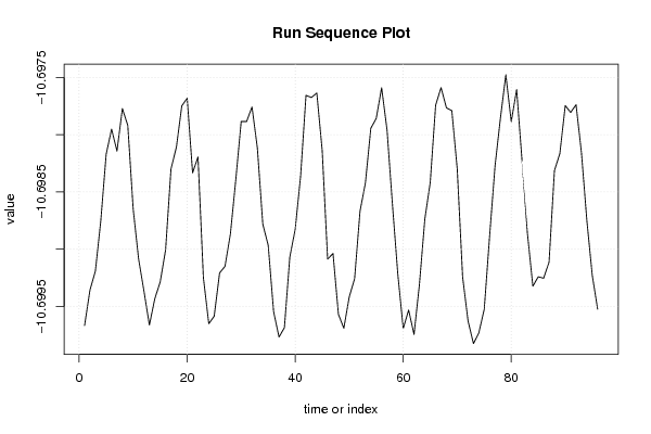
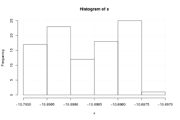
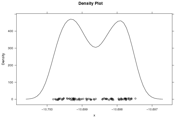
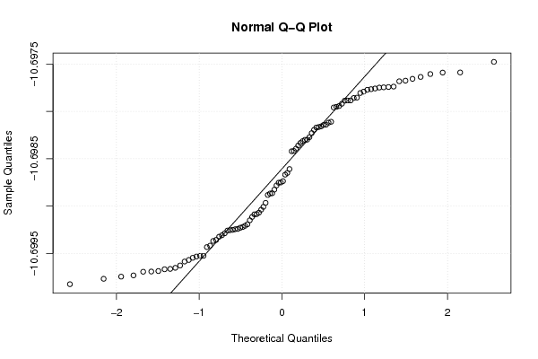
Figures (Output of Computation) | |||||||||||||||||||||||||||||||||||||||||||||||||||||
Input Parameters & R Code | |||||||||||||||||||||||||||||||||||||||||||||||||||||
| Parameters (Session): | |||||||||||||||||||||||||||||||||||||||||||||||||||||
| par1 = 0 ; par2 = 0 ; | |||||||||||||||||||||||||||||||||||||||||||||||||||||
| Parameters (R input): | |||||||||||||||||||||||||||||||||||||||||||||||||||||
| par1 = 0 ; par2 = 0 ; | |||||||||||||||||||||||||||||||||||||||||||||||||||||
| R code (references can be found in the software module): | |||||||||||||||||||||||||||||||||||||||||||||||||||||
par1 <- as.numeric(par1) | |||||||||||||||||||||||||||||||||||||||||||||||||||||