Free Statistics

of Irreproducible Research!

Author's title

Author*The author of this computation has been verified*
R Software Modulerwasp_edauni.wasp
Title produced by softwareUnivariate Explorative Data Analysis
Date of computationThu, 01 Dec 2011 10:29:03 -0500
Cite this page as followsStatistical Computations at FreeStatistics.org, Office for Research Development and Education, URL https://freestatistics.org/blog/index.php?v=date/2011/Dec/01/t1322753371zjnhyaa2l3nyv89.htm/, Retrieved Fri, 19 Apr 2024 07:07:50 +0000
Statistical Computations at FreeStatistics.org, Office for Research Development and Education, URL https://freestatistics.org/blog/index.php?pk=149809, Retrieved Fri, 19 Apr 2024 07:07:50 +0000
QR Codes:

Original text written by user:
IsPrivate?No (this computation is public)
User-defined keywords
Estimated Impact104
Family? (F = Feedback message, R = changed R code, M = changed R Module, P = changed Parameters, D = changed Data)
-     [Univariate Data Series] [web server] [2010-10-19 15:51:23] [b98453cac15ba1066b407e146608df68]
- RMPD  [Classical Decomposition] [Classical Decompo...] [2011-12-01 14:47:37] [15a5dd358825f04074b70fc847ec6454]
- RMPD      [Univariate Explorative Data Analysis] [Sequence plot Wer...] [2011-12-01 15:29:03] [614dd89c388120cee0dd25886939832b] [Current]
Feedback Forum

Post a new message
Dataseries X:
548
563
581
572
519
521
531
540
548
556
551
549
564
586
604
601
545
537
552
563
575
580
575
558
564
581
597
587
536
524
537
536
533
528
516
502
506
518
534
528
478
469
490
493
508
517
514
510
527
542
565
555
499
511
526
532
549
561
557
566
588
620
626
620
573
573
574
580
590
593
597
595
612
628
629
621
569
567
573
584
589
591
595
594
611
613
611
594
543
537
544
555
561
562
555
547
565
578
580
569
507
501
509
510
517
519
512
509
519


Summary of computational transaction
Raw Inputview raw input (R code)
Raw Outputview raw output of R engine
Computing time2 seconds
R Server'Gertrude Mary Cox' @ cox.wessa.net

\begin{tabular}{lllllllll}
\hline
Summary of computational transaction \tabularnewline
Raw Input & view raw input (R code)  \tabularnewline
Raw Output & view raw output of R engine  \tabularnewline
Computing time & 2 seconds \tabularnewline
R Server & 'Gertrude Mary Cox' @ cox.wessa.net \tabularnewline
\hline
\end{tabular}
%Source: https://freestatistics.org/blog/index.php?pk=149809&T=0

[TABLE]
[ROW][C]Summary of computational transaction[/C][/ROW]
[ROW][C]Raw Input[/C][C]view raw input (R code) [/C][/ROW]
[ROW][C]Raw Output[/C][C]view raw output of R engine [/C][/ROW]
[ROW][C]Computing time[/C][C]2 seconds[/C][/ROW]
[ROW][C]R Server[/C][C]'Gertrude Mary Cox' @ cox.wessa.net[/C][/ROW]
[/TABLE]
Source: https://freestatistics.org/blog/index.php?pk=149809&T=0

Globally Unique Identifier (entire table): ba.freestatistics.org/blog/index.php?pk=149809&T=0

As an alternative you can also use a QR Code:  

The GUIDs for individual cells are displayed in the table below:

Summary of computational transaction
Raw Inputview raw input (R code)
Raw Outputview raw output of R engine
Computing time2 seconds
R Server'Gertrude Mary Cox' @ cox.wessa.net


Descriptive Statistics
# observations109
minimum469
Q1527
median556
mean555.266055045872
Q3581
maximum629

\begin{tabular}{lllllllll}
\hline
Descriptive Statistics \tabularnewline
# observations & 109 \tabularnewline
minimum & 469 \tabularnewline
Q1 & 527 \tabularnewline
median & 556 \tabularnewline
mean & 555.266055045872 \tabularnewline
Q3 & 581 \tabularnewline
maximum & 629 \tabularnewline
\hline
\end{tabular}
%Source: https://freestatistics.org/blog/index.php?pk=149809&T=1

[TABLE]
[ROW][C]Descriptive Statistics[/C][/ROW]
[ROW][C]# observations[/C][C]109[/C][/ROW]
[ROW][C]minimum[/C][C]469[/C][/ROW]
[ROW][C]Q1[/C][C]527[/C][/ROW]
[ROW][C]median[/C][C]556[/C][/ROW]
[ROW][C]mean[/C][C]555.266055045872[/C][/ROW]
[ROW][C]Q3[/C][C]581[/C][/ROW]
[ROW][C]maximum[/C][C]629[/C][/ROW]
[/TABLE]
Source: https://freestatistics.org/blog/index.php?pk=149809&T=1

Globally Unique Identifier (entire table): ba.freestatistics.org/blog/index.php?pk=149809&T=1

As an alternative you can also use a QR Code:  

The GUIDs for individual cells are displayed in the table below:

Descriptive Statistics
# observations109
minimum469
Q1527
median556
mean555.266055045872
Q3581
maximum629


Parameters (Session):
par1 = 0 ; par2 = 36 ;
Parameters (R input):
par1 = 0 ; par2 = 36 ;
R code (references can be found in the software module):
par1 <- as.numeric(par1)
par2 <- as.numeric(par2)
x <- as.ts(x)
library(lattice)
bitmap(file='pic1.png')
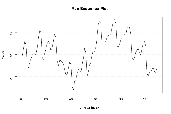
plot(x,type='l',main='Run Sequence Plot',xlab='time or index',ylab='value')
grid()
dev.off()
bitmap(file='pic2.png')
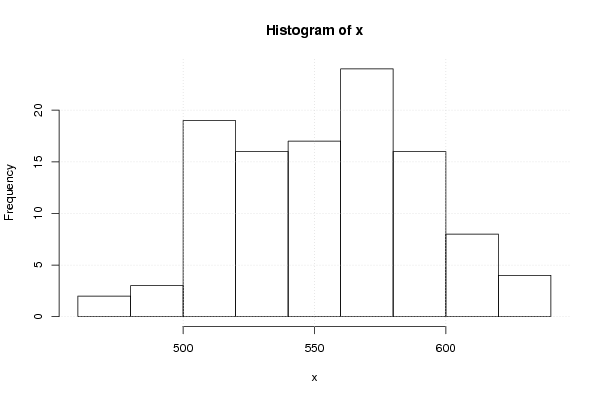
hist(x)
grid()
dev.off()
bitmap(file='pic3.png')
if (par1 > 0)
{
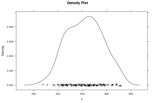
densityplot(~x,col='black',main=paste('Density Plot bw = ',par1),bw=par1)
} else {
densityplot(~x,col='black',main='Density Plot')
}
dev.off()
bitmap(file='pic4.png')
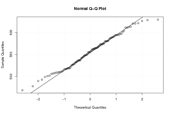
qqnorm(x)
qqline(x)
grid()
dev.off()
if (par2 > 0)
{
bitmap(file='lagplot1.png')
dum <- cbind(lag(x,k=1),x)
dum
dum1 <- dum[2:length(x),]
dum1
z <- as.data.frame(dum1)
z
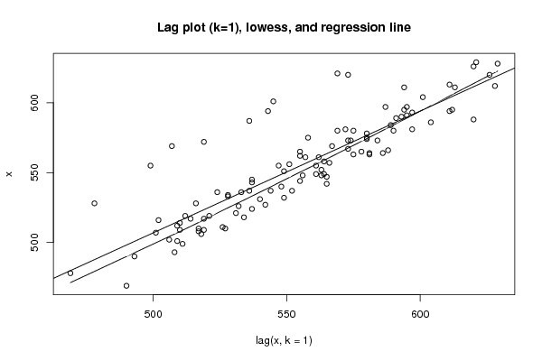
plot(z,main='Lag plot (k=1), lowess, and regression line')
lines(lowess(z))
abline(lm(z))
dev.off()
if (par2 > 1) {
bitmap(file='lagplotpar2.png')
dum <- cbind(lag(x,k=par2),x)
dum
dum1 <- dum[(par2+1):length(x),]
dum1
z <- as.data.frame(dum1)
z
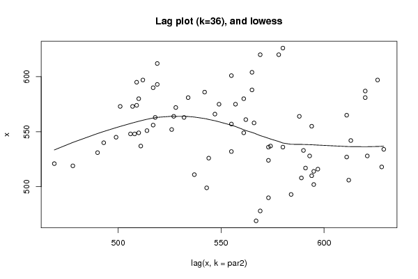
mylagtitle <- 'Lag plot (k='
mylagtitle <- paste(mylagtitle,par2,sep='')
mylagtitle <- paste(mylagtitle,'), and lowess',sep='')
plot(z,main=mylagtitle)
lines(lowess(z))
dev.off()
}
bitmap(file='pic5.png')
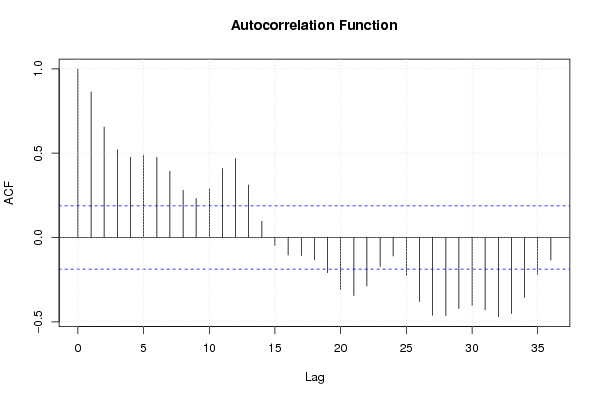
acf(x,lag.max=par2,main='Autocorrelation Function')
grid()
dev.off()
}
summary(x)
load(file='createtable')
a<-table.start()
a<-table.row.start(a)
a<-table.element(a,'Descriptive Statistics',2,TRUE)
a<-table.row.end(a)
a<-table.row.start(a)
a<-table.element(a,'# observations',header=TRUE)
a<-table.element(a,length(x))
a<-table.row.end(a)
a<-table.row.start(a)
a<-table.element(a,'minimum',header=TRUE)
a<-table.element(a,min(x))
a<-table.row.end(a)
a<-table.row.start(a)
a<-table.element(a,'Q1',header=TRUE)
a<-table.element(a,quantile(x,0.25))
a<-table.row.end(a)
a<-table.row.start(a)
a<-table.element(a,'median',header=TRUE)
a<-table.element(a,median(x))
a<-table.row.end(a)
a<-table.row.start(a)
a<-table.element(a,'mean',header=TRUE)
a<-table.element(a,mean(x))
a<-table.row.end(a)
a<-table.row.start(a)
a<-table.element(a,'Q3',header=TRUE)
a<-table.element(a,quantile(x,0.75))
a<-table.row.end(a)
a<-table.row.start(a)
a<-table.element(a,'maximum',header=TRUE)
a<-table.element(a,max(x))
a<-table.row.end(a)
a<-table.end(a)
table.save(a,file='mytable.tab')