Free Statistics
of Irreproducible Research!
Description of Statistical Computation | |||||||||||||||||||||
|---|---|---|---|---|---|---|---|---|---|---|---|---|---|---|---|---|---|---|---|---|---|
| Author's title | |||||||||||||||||||||
| Author | *Unverified author* | ||||||||||||||||||||
| R Software Module | rwasp_meanplot.wasp | ||||||||||||||||||||
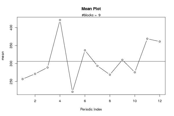
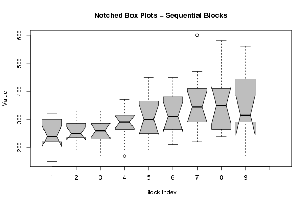
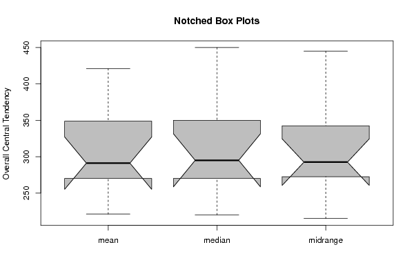
| Title produced by software | Mean Plot | ||||||||||||||||||||
| Date of computation | Tue, 09 Aug 2011 08:29:10 -0400 | ||||||||||||||||||||
| Cite this page as follows | Statistical Computations at FreeStatistics.org, Office for Research Development and Education, URL https://freestatistics.org/blog/index.php?v=date/2011/Aug/09/t13128929942pi6xap73wd0x2o.htm/, Retrieved Mon, 13 May 2024 21:55:11 +0000 | ||||||||||||||||||||
| Statistical Computations at FreeStatistics.org, Office for Research Development and Education, URL https://freestatistics.org/blog/index.php?pk=123479, Retrieved Mon, 13 May 2024 21:55:11 +0000 | |||||||||||||||||||||
| QR Codes: | |||||||||||||||||||||
|
| |||||||||||||||||||||
| Original text written by user: | |||||||||||||||||||||
| IsPrivate? | No (this computation is public) | ||||||||||||||||||||
| User-defined keywords | Nick Verbeke | ||||||||||||||||||||
| Estimated Impact | 131 | ||||||||||||||||||||
Tree of Dependent Computations | |||||||||||||||||||||
| Family? (F = Feedback message, R = changed R code, M = changed R Module, P = changed Parameters, D = changed Data) | |||||||||||||||||||||
| - [Mean Plot] [Mean Plot inschri...] [2011-04-04 14:53:24] [1cb322a33a2333c24d08c776e1f699d5] - D [Mean Plot] [TIJDREEKS B - STA...] [2011-08-09 12:29:10] [af5734c86e7bdbdfefb37d9aed9dbb03] [Current] | |||||||||||||||||||||
| Feedback Forum | |||||||||||||||||||||
Post a new message | |||||||||||||||||||||
Dataset | |||||||||||||||||||||
| Dataseries X: | |||||||||||||||||||||
240 150 290 210 240 240 310 310 190 230 260 320 270 250 240 250 230 230 240 300 190 270 300 330 230 260 300 330 190 260 240 270 170 230 270 320 190 300 310 360 170 280 270 260 280 300 320 370 210 310 290 450 190 290 280 310 340 220 390 410 250 310 280 450 210 390 300 310 370 250 440 360 290 300 340 600 220 410 360 250 410 290 470 350 330 250 270 580 260 450 320 240 420 380 400 370 300 310 280 560 280 480 320 170 420 310 470 420 | |||||||||||||||||||||
Tables (Output of Computation) | |||||||||||||||||||||
| |||||||||||||||||||||
Figures (Output of Computation) | |||||||||||||||||||||
Input Parameters & R Code | |||||||||||||||||||||
| Parameters (Session): | |||||||||||||||||||||
| par1 = 12 ; | |||||||||||||||||||||
| Parameters (R input): | |||||||||||||||||||||
| par1 = 12 ; | |||||||||||||||||||||
| R code (references can be found in the software module): | |||||||||||||||||||||
par1 <- as.numeric(par1) | |||||||||||||||||||||