Free Statistics
of Irreproducible Research!
Description of Statistical Computation | |||||||||||||||||||||
|---|---|---|---|---|---|---|---|---|---|---|---|---|---|---|---|---|---|---|---|---|---|
| Author's title | |||||||||||||||||||||
| Author | *Unverified author* | ||||||||||||||||||||
| R Software Module | rwasp_meanplot.wasp | ||||||||||||||||||||
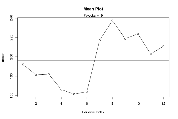
| Title produced by software | Mean Plot | ||||||||||||||||||||
| Date of computation | Wed, 06 Apr 2011 11:40:41 +0000 | ||||||||||||||||||||
| Cite this page as follows | Statistical Computations at FreeStatistics.org, Office for Research Development and Education, URL https://freestatistics.org/blog/index.php?v=date/2011/Apr/06/t130208996718v0oy3i5k68rze.htm/, Retrieved Thu, 09 May 2024 18:50:22 +0000 | ||||||||||||||||||||
| Statistical Computations at FreeStatistics.org, Office for Research Development and Education, URL https://freestatistics.org/blog/index.php?pk=120345, Retrieved Thu, 09 May 2024 18:50:22 +0000 | |||||||||||||||||||||
| QR Codes: | |||||||||||||||||||||
|
| |||||||||||||||||||||
| Original text written by user: | |||||||||||||||||||||
| IsPrivate? | No (this computation is public) | ||||||||||||||||||||
| User-defined keywords | KDGP1W52 | ||||||||||||||||||||
| Estimated Impact | 185 | ||||||||||||||||||||
Tree of Dependent Computations | |||||||||||||||||||||
| Family? (F = Feedback message, R = changed R code, M = changed R Module, P = changed Parameters, D = changed Data) | |||||||||||||||||||||
| - [Mean Plot] [Opgave 6 stap 2 -...] [2011-04-04 15:02:35] [c5099653210d8fa3a7a4ff12c906fbc3] - R [Mean Plot] [KDGP1W51] [2011-04-06 11:32:06] [3f6343f1a4fd4c523f66adbf44782a9f] - R D [Mean Plot] [KDGP1W52] [2011-04-06 11:40:41] [19a61d0bd13d2baa9a7acd2fea0b77e4] [Current] | |||||||||||||||||||||
| Feedback Forum | |||||||||||||||||||||
Post a new message | |||||||||||||||||||||
Dataset | |||||||||||||||||||||
| Dataseries X: | |||||||||||||||||||||
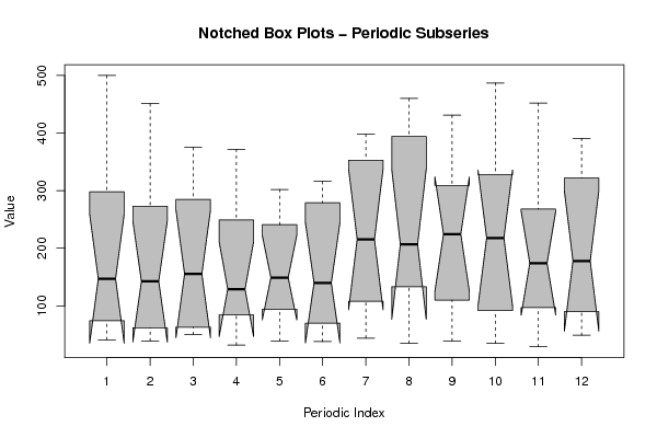
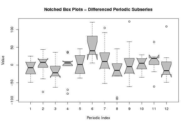
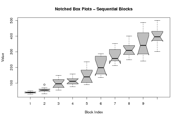
41 39 50 40 43 38 44 35 39 35 29 49 50 59 63 32 39 47 53 60 57 52 70 90 74 62 55 84 94 70 108 139 120 97 126 149 158 124 140 109 114 77 120 133 110 92 97 78 99 107 112 90 98 125 155 190 236 189 174 178 136 161 171 149 184 155 276 224 213 279 268 287 238 213 257 293 212 246 353 339 308 247 257 322 298 273 312 249 286 279 309 401 309 328 353 354 327 324 285 243 241 287 355 460 364 487 452 391 500 451 375 372 302 316 398 394 431 431 | |||||||||||||||||||||
Tables (Output of Computation) | |||||||||||||||||||||
| |||||||||||||||||||||
Figures (Output of Computation) | |||||||||||||||||||||
Input Parameters & R Code | |||||||||||||||||||||
| Parameters (Session): | |||||||||||||||||||||
| par1 = 12 ; | |||||||||||||||||||||
| Parameters (R input): | |||||||||||||||||||||
| par1 = 12 ; | |||||||||||||||||||||
| R code (references can be found in the software module): | |||||||||||||||||||||
par1 <- as.numeric(par1) | |||||||||||||||||||||