Free Statistics
of Irreproducible Research!
Description of Statistical Computation | |||||||||||||||||||||||||||||||||||||||||||||||||||||||||||||||||||||||||||||||||||||||||||||||||||||||||||||||||||||||||||||||||||||||||||||||||||||||||||||||||||||||||||||||
|---|---|---|---|---|---|---|---|---|---|---|---|---|---|---|---|---|---|---|---|---|---|---|---|---|---|---|---|---|---|---|---|---|---|---|---|---|---|---|---|---|---|---|---|---|---|---|---|---|---|---|---|---|---|---|---|---|---|---|---|---|---|---|---|---|---|---|---|---|---|---|---|---|---|---|---|---|---|---|---|---|---|---|---|---|---|---|---|---|---|---|---|---|---|---|---|---|---|---|---|---|---|---|---|---|---|---|---|---|---|---|---|---|---|---|---|---|---|---|---|---|---|---|---|---|---|---|---|---|---|---|---|---|---|---|---|---|---|---|---|---|---|---|---|---|---|---|---|---|---|---|---|---|---|---|---|---|---|---|---|---|---|---|---|---|---|---|---|---|---|---|---|---|---|---|---|
| Author's title | |||||||||||||||||||||||||||||||||||||||||||||||||||||||||||||||||||||||||||||||||||||||||||||||||||||||||||||||||||||||||||||||||||||||||||||||||||||||||||||||||||||||||||||||
| Author | *The author of this computation has been verified* | ||||||||||||||||||||||||||||||||||||||||||||||||||||||||||||||||||||||||||||||||||||||||||||||||||||||||||||||||||||||||||||||||||||||||||||||||||||||||||||||||||||||||||||||
| R Software Module | rwasp_One Factor ANOVA.wasp | ||||||||||||||||||||||||||||||||||||||||||||||||||||||||||||||||||||||||||||||||||||||||||||||||||||||||||||||||||||||||||||||||||||||||||||||||||||||||||||||||||||||||||||||
| Title produced by software | One-Way-Between-Groups ANOVA- Free Statistics Software (Calculator) | ||||||||||||||||||||||||||||||||||||||||||||||||||||||||||||||||||||||||||||||||||||||||||||||||||||||||||||||||||||||||||||||||||||||||||||||||||||||||||||||||||||||||||||||
| Date of computation | Thu, 28 Oct 2010 20:11:30 +0000 | ||||||||||||||||||||||||||||||||||||||||||||||||||||||||||||||||||||||||||||||||||||||||||||||||||||||||||||||||||||||||||||||||||||||||||||||||||||||||||||||||||||||||||||||
| Cite this page as follows | Statistical Computations at FreeStatistics.org, Office for Research Development and Education, URL https://freestatistics.org/blog/index.php?v=date/2010/Oct/28/t1288296619y98xtk1m62ar8lx.htm/, Retrieved Fri, 03 May 2024 15:53:37 +0000 | ||||||||||||||||||||||||||||||||||||||||||||||||||||||||||||||||||||||||||||||||||||||||||||||||||||||||||||||||||||||||||||||||||||||||||||||||||||||||||||||||||||||||||||||
| Statistical Computations at FreeStatistics.org, Office for Research Development and Education, URL https://freestatistics.org/blog/index.php?pk=89903, Retrieved Fri, 03 May 2024 15:53:37 +0000 | |||||||||||||||||||||||||||||||||||||||||||||||||||||||||||||||||||||||||||||||||||||||||||||||||||||||||||||||||||||||||||||||||||||||||||||||||||||||||||||||||||||||||||||||
| QR Codes: | |||||||||||||||||||||||||||||||||||||||||||||||||||||||||||||||||||||||||||||||||||||||||||||||||||||||||||||||||||||||||||||||||||||||||||||||||||||||||||||||||||||||||||||||
|
| |||||||||||||||||||||||||||||||||||||||||||||||||||||||||||||||||||||||||||||||||||||||||||||||||||||||||||||||||||||||||||||||||||||||||||||||||||||||||||||||||||||||||||||||
| Original text written by user: | |||||||||||||||||||||||||||||||||||||||||||||||||||||||||||||||||||||||||||||||||||||||||||||||||||||||||||||||||||||||||||||||||||||||||||||||||||||||||||||||||||||||||||||||
| IsPrivate? | No (this computation is public) | ||||||||||||||||||||||||||||||||||||||||||||||||||||||||||||||||||||||||||||||||||||||||||||||||||||||||||||||||||||||||||||||||||||||||||||||||||||||||||||||||||||||||||||||
| User-defined keywords | |||||||||||||||||||||||||||||||||||||||||||||||||||||||||||||||||||||||||||||||||||||||||||||||||||||||||||||||||||||||||||||||||||||||||||||||||||||||||||||||||||||||||||||||
| Estimated Impact | 206 | ||||||||||||||||||||||||||||||||||||||||||||||||||||||||||||||||||||||||||||||||||||||||||||||||||||||||||||||||||||||||||||||||||||||||||||||||||||||||||||||||||||||||||||||
Tree of Dependent Computations | |||||||||||||||||||||||||||||||||||||||||||||||||||||||||||||||||||||||||||||||||||||||||||||||||||||||||||||||||||||||||||||||||||||||||||||||||||||||||||||||||||||||||||||||
| Family? (F = Feedback message, R = changed R code, M = changed R Module, P = changed Parameters, D = changed Data) | |||||||||||||||||||||||||||||||||||||||||||||||||||||||||||||||||||||||||||||||||||||||||||||||||||||||||||||||||||||||||||||||||||||||||||||||||||||||||||||||||||||||||||||||
| - [One-Way-Between-Groups ANOVA- Free Statistics Software (Calculator)] [Golfballs] [2010-10-25 12:27:51] [b98453cac15ba1066b407e146608df68] F PD [One-Way-Between-Groups ANOVA- Free Statistics Software (Calculator)] [WS5 Q6.1 KT] [2010-10-28 19:53:10] [afe9379cca749d06b3d6872e02cc47ed] F D [One-Way-Between-Groups ANOVA- Free Statistics Software (Calculator)] [ws5 Q6.2 LT] [2010-10-28 20:11:30] [aa6b599ccd367bc74fed0d8f67004a46] [Current] F [One-Way-Between-Groups ANOVA- Free Statistics Software (Calculator)] [Taak 6: lange ter...] [2010-10-29 18:12:48] [74deae64b71f9d77c839af86f7c687b5] F R P [One-Way-Between-Groups ANOVA- Free Statistics Software (Calculator)] [WS 5 Q 6] [2010-11-02 16:59:42] [4f85667043e8913570b3eb8f368f82b2] - [One-Way-Between-Groups ANOVA- Free Statistics Software (Calculator)] [] [2010-11-03 06:51:59] [b64b273f7a25c5bb07ff2f026b8ce952] - [One-Way-Between-Groups ANOVA- Free Statistics Software (Calculator)] [] [2010-11-03 06:54:41] [b64b273f7a25c5bb07ff2f026b8ce952] - R [One-Way-Between-Groups ANOVA- Free Statistics Software (Calculator)] [ws 5 - opdracht 6] [2011-11-04 15:04:06] [4b648d52023f19d55c572f0eddd72b1f] - R PD [One-Way-Between-Groups ANOVA- Free Statistics Software (Calculator)] [WS5 taak 6] [2012-10-29 16:52:49] [ebc10d82be597731a57172229e4f44b7] - R P [One-Way-Between-Groups ANOVA- Free Statistics Software (Calculator)] [Q6 - lange termijn] [2012-10-29 20:59:13] [74be16979710d4c4e7c6647856088456] - R [One-Way-Between-Groups ANOVA- Free Statistics Software (Calculator)] [] [2012-10-30 18:16:35] [74be16979710d4c4e7c6647856088456] - R [One-Way-Between-Groups ANOVA- Free Statistics Software (Calculator)] [WS 5 vraag 6 ] [2013-11-03 14:44:57] [16ce55620e4b91ec00a4b56aea2a2582] | |||||||||||||||||||||||||||||||||||||||||||||||||||||||||||||||||||||||||||||||||||||||||||||||||||||||||||||||||||||||||||||||||||||||||||||||||||||||||||||||||||||||||||||||
| Feedback Forum | |||||||||||||||||||||||||||||||||||||||||||||||||||||||||||||||||||||||||||||||||||||||||||||||||||||||||||||||||||||||||||||||||||||||||||||||||||||||||||||||||||||||||||||||
Post a new message | |||||||||||||||||||||||||||||||||||||||||||||||||||||||||||||||||||||||||||||||||||||||||||||||||||||||||||||||||||||||||||||||||||||||||||||||||||||||||||||||||||||||||||||||
Dataset | |||||||||||||||||||||||||||||||||||||||||||||||||||||||||||||||||||||||||||||||||||||||||||||||||||||||||||||||||||||||||||||||||||||||||||||||||||||||||||||||||||||||||||||||
| Dataseries X: | |||||||||||||||||||||||||||||||||||||||||||||||||||||||||||||||||||||||||||||||||||||||||||||||||||||||||||||||||||||||||||||||||||||||||||||||||||||||||||||||||||||||||||||||
-1 'T' -1 'T' 1 'T' 0 'T' 0 'T' 0 'T' 0 'T' 1 'T' 1 'T' -1 'T' 0 'T' 1 'T' 1 'T' 0 'T' 0 'T' -1 'T' 0 'T' 1 'T' 1 'T' 0 'T' -1 'T' 0 'T' 0 'T' 0 'T' 0 'T' -1 'T' -1 'T' 1 'T' 1 'T' -1 'T' 1 'E' 1 'E' 0 'E' 0 'E' 0 'E' -1 'E' 0 'E' 1 'E' 1 'E' 0 'E' -1 'E' 0 'E' 0 'E' 1 'E' 0 'E' 1 'E' 0 'E' 1 'E' 1 'E' 0 'E' 1 'E' 0 'E' 0 'E' 0 'E' 1 'E' 0 'E' 1 'E' 0 'E' 0 'E' 0 'E' 0 'S' 0 'S' 0 'S' 0 'S' 0 'S' 0 'S' 1 'S' 0 'S' 0 'S' 0 'S' 1 'S' 1 'S' 1 'S' 0 'S' 1 'S' 0 'S' 1 'S' -1 'S' 0 'S' 1 'S' 0 'S' 0 'S' 0 'S' 0 'S' 0 'S' -1 'S' 1 'S' 0 'S' 1 'S' 0 'S' | |||||||||||||||||||||||||||||||||||||||||||||||||||||||||||||||||||||||||||||||||||||||||||||||||||||||||||||||||||||||||||||||||||||||||||||||||||||||||||||||||||||||||||||||
Tables (Output of Computation) | |||||||||||||||||||||||||||||||||||||||||||||||||||||||||||||||||||||||||||||||||||||||||||||||||||||||||||||||||||||||||||||||||||||||||||||||||||||||||||||||||||||||||||||||
| |||||||||||||||||||||||||||||||||||||||||||||||||||||||||||||||||||||||||||||||||||||||||||||||||||||||||||||||||||||||||||||||||||||||||||||||||||||||||||||||||||||||||||||||
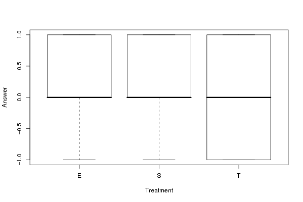
Figures (Output of Computation) | |||||||||||||||||||||||||||||||||||||||||||||||||||||||||||||||||||||||||||||||||||||||||||||||||||||||||||||||||||||||||||||||||||||||||||||||||||||||||||||||||||||||||||||||
Input Parameters & R Code | |||||||||||||||||||||||||||||||||||||||||||||||||||||||||||||||||||||||||||||||||||||||||||||||||||||||||||||||||||||||||||||||||||||||||||||||||||||||||||||||||||||||||||||||
| Parameters (Session): | |||||||||||||||||||||||||||||||||||||||||||||||||||||||||||||||||||||||||||||||||||||||||||||||||||||||||||||||||||||||||||||||||||||||||||||||||||||||||||||||||||||||||||||||
| par1 = 1 ; par2 = 2 ; par3 = TRUE ; | |||||||||||||||||||||||||||||||||||||||||||||||||||||||||||||||||||||||||||||||||||||||||||||||||||||||||||||||||||||||||||||||||||||||||||||||||||||||||||||||||||||||||||||||
| Parameters (R input): | |||||||||||||||||||||||||||||||||||||||||||||||||||||||||||||||||||||||||||||||||||||||||||||||||||||||||||||||||||||||||||||||||||||||||||||||||||||||||||||||||||||||||||||||
| par1 = 1 ; par2 = 2 ; par3 = TRUE ; | |||||||||||||||||||||||||||||||||||||||||||||||||||||||||||||||||||||||||||||||||||||||||||||||||||||||||||||||||||||||||||||||||||||||||||||||||||||||||||||||||||||||||||||||
| R code (references can be found in the software module): | |||||||||||||||||||||||||||||||||||||||||||||||||||||||||||||||||||||||||||||||||||||||||||||||||||||||||||||||||||||||||||||||||||||||||||||||||||||||||||||||||||||||||||||||
cat1 <- as.numeric(par1) # | |||||||||||||||||||||||||||||||||||||||||||||||||||||||||||||||||||||||||||||||||||||||||||||||||||||||||||||||||||||||||||||||||||||||||||||||||||||||||||||||||||||||||||||||