Free Statistics
of Irreproducible Research!
Description of Statistical Computation | |||||||||||||||||||||||||||||||||||||||
|---|---|---|---|---|---|---|---|---|---|---|---|---|---|---|---|---|---|---|---|---|---|---|---|---|---|---|---|---|---|---|---|---|---|---|---|---|---|---|---|
| Author's title | |||||||||||||||||||||||||||||||||||||||
| Author | *The author of this computation has been verified* | ||||||||||||||||||||||||||||||||||||||
| R Software Module | rwasp_fitdistrnorm.wasp | ||||||||||||||||||||||||||||||||||||||
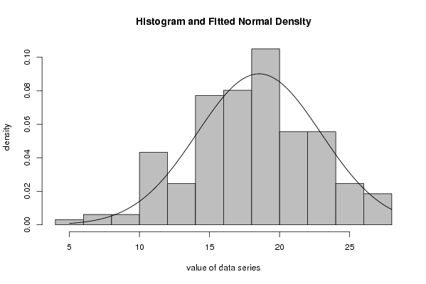
| Title produced by software | Maximum-likelihood Fitting - Normal Distribution | ||||||||||||||||||||||||||||||||||||||
| Date of computation | Tue, 19 Oct 2010 15:35:19 +0000 | ||||||||||||||||||||||||||||||||||||||
| Cite this page as follows | Statistical Computations at FreeStatistics.org, Office for Research Development and Education, URL https://freestatistics.org/blog/index.php?v=date/2010/Oct/19/t1287502441ewh0sdmlplce7kh.htm/, Retrieved Sun, 28 Apr 2024 21:27:05 +0000 | ||||||||||||||||||||||||||||||||||||||
| Statistical Computations at FreeStatistics.org, Office for Research Development and Education, URL https://freestatistics.org/blog/index.php?pk=86653, Retrieved Sun, 28 Apr 2024 21:27:05 +0000 | |||||||||||||||||||||||||||||||||||||||
| QR Codes: | |||||||||||||||||||||||||||||||||||||||
|
| |||||||||||||||||||||||||||||||||||||||
| Original text written by user: | |||||||||||||||||||||||||||||||||||||||
| IsPrivate? | No (this computation is public) | ||||||||||||||||||||||||||||||||||||||
| User-defined keywords | |||||||||||||||||||||||||||||||||||||||
| Estimated Impact | 106 | ||||||||||||||||||||||||||||||||||||||
Tree of Dependent Computations | |||||||||||||||||||||||||||||||||||||||
| Family? (F = Feedback message, R = changed R code, M = changed R Module, P = changed Parameters, D = changed Data) | |||||||||||||||||||||||||||||||||||||||
| - [Maximum-likelihood Fitting - Normal Distribution] [Intrinsic Motivat...] [2010-10-12 11:57:21] [b98453cac15ba1066b407e146608df68] F PD [Maximum-likelihood Fitting - Normal Distribution] [] [2010-10-19 15:35:19] [6b31f806e9ccc1f74a26091056f791cb] [Current] | |||||||||||||||||||||||||||||||||||||||
| Feedback Forum | |||||||||||||||||||||||||||||||||||||||
Post a new message | |||||||||||||||||||||||||||||||||||||||
Dataset | |||||||||||||||||||||||||||||||||||||||
| Dataseries X: | |||||||||||||||||||||||||||||||||||||||
21 16 19 18 16 23 17 12 19 16 19 20 13 20 27 17 8 25 26 13 19 15 5 16 14 24 24 9 19 19 25 19 18 15 12 21 12 15 28 25 19 20 24 26 25 12 12 15 17 14 16 11 20 11 22 20 19 17 21 23 18 17 27 25 19 22 24 20 19 11 22 22 16 20 24 16 16 22 24 16 27 11 21 20 20 27 20 12 8 21 18 24 16 18 20 20 19 17 16 26 15 22 17 23 21 19 14 17 12 24 18 20 16 20 22 12 16 17 22 12 14 23 15 17 28 20 23 13 18 23 19 23 12 16 23 13 22 18 23 20 10 17 18 15 23 17 17 22 20 20 19 18 22 20 22 18 16 16 16 16 17 18 | |||||||||||||||||||||||||||||||||||||||
Tables (Output of Computation) | |||||||||||||||||||||||||||||||||||||||
| |||||||||||||||||||||||||||||||||||||||
Figures (Output of Computation) | |||||||||||||||||||||||||||||||||||||||
Input Parameters & R Code | |||||||||||||||||||||||||||||||||||||||
| Parameters (Session): | |||||||||||||||||||||||||||||||||||||||
| par1 = 8 ; par2 = 0 ; | |||||||||||||||||||||||||||||||||||||||
| Parameters (R input): | |||||||||||||||||||||||||||||||||||||||
| par1 = 8 ; par2 = 0 ; | |||||||||||||||||||||||||||||||||||||||
| R code (references can be found in the software module): | |||||||||||||||||||||||||||||||||||||||
library(MASS) | |||||||||||||||||||||||||||||||||||||||