Free Statistics
of Irreproducible Research!
Description of Statistical Computation | |||||||||||||||||||||||||||||||||||||||||||||||||||||||||||||||||||||||||||||||||||||||||||||||||||||||||||||||||||||||||||||||||||||||||||||||||||||||||||||||||||||||||||||||||||||||||||||||||||||||||
|---|---|---|---|---|---|---|---|---|---|---|---|---|---|---|---|---|---|---|---|---|---|---|---|---|---|---|---|---|---|---|---|---|---|---|---|---|---|---|---|---|---|---|---|---|---|---|---|---|---|---|---|---|---|---|---|---|---|---|---|---|---|---|---|---|---|---|---|---|---|---|---|---|---|---|---|---|---|---|---|---|---|---|---|---|---|---|---|---|---|---|---|---|---|---|---|---|---|---|---|---|---|---|---|---|---|---|---|---|---|---|---|---|---|---|---|---|---|---|---|---|---|---|---|---|---|---|---|---|---|---|---|---|---|---|---|---|---|---|---|---|---|---|---|---|---|---|---|---|---|---|---|---|---|---|---|---|---|---|---|---|---|---|---|---|---|---|---|---|---|---|---|---|---|---|---|---|---|---|---|---|---|---|---|---|---|---|---|---|---|---|---|---|---|---|---|---|---|---|---|---|---|
| Author's title | |||||||||||||||||||||||||||||||||||||||||||||||||||||||||||||||||||||||||||||||||||||||||||||||||||||||||||||||||||||||||||||||||||||||||||||||||||||||||||||||||||||||||||||||||||||||||||||||||||||||||
| Author | *The author of this computation has been verified* | ||||||||||||||||||||||||||||||||||||||||||||||||||||||||||||||||||||||||||||||||||||||||||||||||||||||||||||||||||||||||||||||||||||||||||||||||||||||||||||||||||||||||||||||||||||||||||||||||||||||||
| R Software Module | rwasp_notchedbox1.wasp | ||||||||||||||||||||||||||||||||||||||||||||||||||||||||||||||||||||||||||||||||||||||||||||||||||||||||||||||||||||||||||||||||||||||||||||||||||||||||||||||||||||||||||||||||||||||||||||||||||||||||
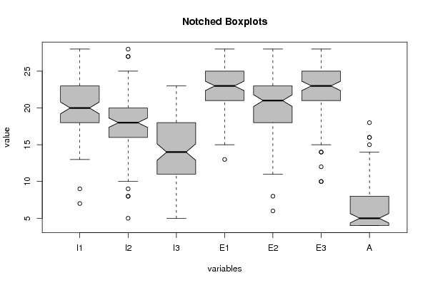
| Title produced by software | Notched Boxplots | ||||||||||||||||||||||||||||||||||||||||||||||||||||||||||||||||||||||||||||||||||||||||||||||||||||||||||||||||||||||||||||||||||||||||||||||||||||||||||||||||||||||||||||||||||||||||||||||||||||||||
| Date of computation | Tue, 19 Oct 2010 09:22:21 +0000 | ||||||||||||||||||||||||||||||||||||||||||||||||||||||||||||||||||||||||||||||||||||||||||||||||||||||||||||||||||||||||||||||||||||||||||||||||||||||||||||||||||||||||||||||||||||||||||||||||||||||||
| Cite this page as follows | Statistical Computations at FreeStatistics.org, Office for Research Development and Education, URL https://freestatistics.org/blog/index.php?v=date/2010/Oct/19/t1287480076qcs5qb59kstc6kx.htm/, Retrieved Sun, 28 Apr 2024 22:40:39 +0000 | ||||||||||||||||||||||||||||||||||||||||||||||||||||||||||||||||||||||||||||||||||||||||||||||||||||||||||||||||||||||||||||||||||||||||||||||||||||||||||||||||||||||||||||||||||||||||||||||||||||||||
| Statistical Computations at FreeStatistics.org, Office for Research Development and Education, URL https://freestatistics.org/blog/index.php?pk=86052, Retrieved Sun, 28 Apr 2024 22:40:39 +0000 | |||||||||||||||||||||||||||||||||||||||||||||||||||||||||||||||||||||||||||||||||||||||||||||||||||||||||||||||||||||||||||||||||||||||||||||||||||||||||||||||||||||||||||||||||||||||||||||||||||||||||
| QR Codes: | |||||||||||||||||||||||||||||||||||||||||||||||||||||||||||||||||||||||||||||||||||||||||||||||||||||||||||||||||||||||||||||||||||||||||||||||||||||||||||||||||||||||||||||||||||||||||||||||||||||||||
|
| |||||||||||||||||||||||||||||||||||||||||||||||||||||||||||||||||||||||||||||||||||||||||||||||||||||||||||||||||||||||||||||||||||||||||||||||||||||||||||||||||||||||||||||||||||||||||||||||||||||||||
| Original text written by user: | |||||||||||||||||||||||||||||||||||||||||||||||||||||||||||||||||||||||||||||||||||||||||||||||||||||||||||||||||||||||||||||||||||||||||||||||||||||||||||||||||||||||||||||||||||||||||||||||||||||||||
| IsPrivate? | No (this computation is public) | ||||||||||||||||||||||||||||||||||||||||||||||||||||||||||||||||||||||||||||||||||||||||||||||||||||||||||||||||||||||||||||||||||||||||||||||||||||||||||||||||||||||||||||||||||||||||||||||||||||||||
| User-defined keywords | |||||||||||||||||||||||||||||||||||||||||||||||||||||||||||||||||||||||||||||||||||||||||||||||||||||||||||||||||||||||||||||||||||||||||||||||||||||||||||||||||||||||||||||||||||||||||||||||||||||||||
| Estimated Impact | 187 | ||||||||||||||||||||||||||||||||||||||||||||||||||||||||||||||||||||||||||||||||||||||||||||||||||||||||||||||||||||||||||||||||||||||||||||||||||||||||||||||||||||||||||||||||||||||||||||||||||||||||
Tree of Dependent Computations | |||||||||||||||||||||||||||||||||||||||||||||||||||||||||||||||||||||||||||||||||||||||||||||||||||||||||||||||||||||||||||||||||||||||||||||||||||||||||||||||||||||||||||||||||||||||||||||||||||||||||
| Family? (F = Feedback message, R = changed R code, M = changed R Module, P = changed Parameters, D = changed Data) | |||||||||||||||||||||||||||||||||||||||||||||||||||||||||||||||||||||||||||||||||||||||||||||||||||||||||||||||||||||||||||||||||||||||||||||||||||||||||||||||||||||||||||||||||||||||||||||||||||||||||
| - [Notched Boxplots] [Academic Motivati...] [2010-10-12 12:51:42] [b98453cac15ba1066b407e146608df68] F D [Notched Boxplots] [WS3 Q4 - Males] [2010-10-19 09:22:21] [aa6b599ccd367bc74fed0d8f67004a46] [Current] - D [Notched Boxplots] [WS3 Q4 - Females] [2010-10-19 09:24:09] [afe9379cca749d06b3d6872e02cc47ed] - P [Notched Boxplots] [] [2010-10-19 14:29:16] [b64b273f7a25c5bb07ff2f026b8ce952] - R [Notched Boxplots] [WS3 - 4 vrouwen] [2012-10-15 08:51:09] [74be16979710d4c4e7c6647856088456] - R [Notched Boxplots] [Academic motivati...] [2012-10-15 15:11:25] [74be16979710d4c4e7c6647856088456] - PD [Notched Boxplots] [Mannen (1)] [2010-10-19 10:35:10] [945bcebba5e7ac34a41d6888338a1ba9] F D [Notched Boxplots] [Mannen (1)] [2010-10-19 10:47:39] [945bcebba5e7ac34a41d6888338a1ba9] F [Notched Boxplots] [Vrouwen (2)] [2010-10-19 10:50:14] [945bcebba5e7ac34a41d6888338a1ba9] - [Notched Boxplots] [] [2010-10-19 15:53:49] [f72e5115d7374b3b3f29ba3966e5379d] - [Notched Boxplots] [] [2010-10-19 15:52:56] [f72e5115d7374b3b3f29ba3966e5379d] - P [Notched Boxplots] [] [2010-10-19 14:25:33] [b64b273f7a25c5bb07ff2f026b8ce952] - R PD [Notched Boxplots] [Mannen Boxplot w3] [2012-10-14 08:00:48] [87b90d598c60c012567ac118c8f3a654] - M [Notched Boxplots] [WS 3 - Q 4.2] [2012-10-16 09:38:38] [0604709baf8ca89a71bc0fcadc3cdffd] - R [Notched Boxplots] [WS3 - 4 mannen] [2012-10-15 08:50:24] [74be16979710d4c4e7c6647856088456] - R D [Notched Boxplots] [Academic motivati...] [2012-10-15 15:08:47] [74be16979710d4c4e7c6647856088456] | |||||||||||||||||||||||||||||||||||||||||||||||||||||||||||||||||||||||||||||||||||||||||||||||||||||||||||||||||||||||||||||||||||||||||||||||||||||||||||||||||||||||||||||||||||||||||||||||||||||||||
| Feedback Forum | |||||||||||||||||||||||||||||||||||||||||||||||||||||||||||||||||||||||||||||||||||||||||||||||||||||||||||||||||||||||||||||||||||||||||||||||||||||||||||||||||||||||||||||||||||||||||||||||||||||||||
Post a new message | |||||||||||||||||||||||||||||||||||||||||||||||||||||||||||||||||||||||||||||||||||||||||||||||||||||||||||||||||||||||||||||||||||||||||||||||||||||||||||||||||||||||||||||||||||||||||||||||||||||||||
Dataset | |||||||||||||||||||||||||||||||||||||||||||||||||||||||||||||||||||||||||||||||||||||||||||||||||||||||||||||||||||||||||||||||||||||||||||||||||||||||||||||||||||||||||||||||||||||||||||||||||||||||||
| Dataseries X: | |||||||||||||||||||||||||||||||||||||||||||||||||||||||||||||||||||||||||||||||||||||||||||||||||||||||||||||||||||||||||||||||||||||||||||||||||||||||||||||||||||||||||||||||||||||||||||||||||||||||||
7 5 6 20 14 21 4 9 18 9 23 26 25 5 13 8 9 24 22 28 4 15 12 9 20 18 24 16 15 18 9 13 20 10 4 15 12 10 18 18 27 8 16 11 10 23 16 10 4 16 11 9 24 20 23 5 16 16 14 18 22 18 8 16 16 14 17 20 18 8 16 20 13 25 24 24 7 16 16 12 21 27 27 7 16 15 7 24 22 21 5 16 19 15 20 18 23 7 16 16 16 19 27 25 16 17 14 11 26 23 27 5 17 19 18 20 18 17 18 17 12 11 19 20 22 14 17 17 18 15 14 15 12 18 12 7 23 25 28 4 18 19 15 26 21 27 7 18 16 17 22 15 21 9 18 20 10 22 21 21 5 18 17 12 20 22 23 6 18 11 12 22 13 21 5 18 19 15 20 21 20 10 18 20 12 20 20 21 6 18 10 8 21 15 24 6 18 16 18 25 23 20 6 19 19 18 22 18 20 6 19 13 14 27 14 22 4 19 9 5 20 8 27 4 19 11 14 23 13 23 4 19 8 14 25 6 28 8 19 20 13 25 22 25 7 19 17 14 21 18 20 6 19 14 18 21 15 21 10 19 23 18 22 24 24 8 20 16 15 24 17 20 4 20 16 8 24 20 24 8 20 24 14 22 26 22 6 20 19 14 24 20 21 4 20 20 12 25 22 22 4 20 21 13 21 21 26 8 20 16 12 18 18 17 4 20 17 14 25 21 24 8 20 13 11 26 17 24 6 20 17 17 26 22 24 7 20 17 10 19 18 21 4 20 16 17 22 18 21 6 20 18 17 20 16 18 4 21 15 19 24 24 28 7 21 18 20 18 24 12 15 21 17 18 25 17 22 6 21 27 16 23 20 21 4 21 22 19 28 19 28 4 21 15 11 24 23 23 4 21 22 14 26 26 22 11 21 19 12 22 19 26 5 22 12 20 27 22 20 8 22 16 14 23 18 23 4 22 13 15 25 23 25 8 22 19 17 23 21 21 4 22 25 15 26 23 22 4 22 20 16 25 26 28 5 22 19 18 24 24 25 4 22 16 13 25 23 22 6 22 23 19 25 24 24 4 22 24 17 23 22 23 4 22 20 10 24 25 23 5 22 18 12 25 23 28 6 22 16 13 25 23 22 6 23 19 15 24 23 21 4 23 20 10 23 21 26 4 23 18 19 26 20 21 4 23 18 8 28 27 26 4 23 13 14 22 11 23 8 23 20 20 23 23 22 8 24 20 8 28 11 24 4 24 17 10 25 14 24 4 24 18 9 17 20 25 4 24 20 23 25 23 19 10 24 24 22 25 26 26 5 24 20 16 26 22 27 5 24 17 18 21 21 24 8 24 17 19 23 20 20 6 24 12 15 28 11 27 4 25 23 19 27 28 22 4 25 24 17 23 24 14 4 25 24 17 23 24 14 4 25 22 20 28 24 25 4 25 23 22 23 26 22 4 25 23 22 27 20 26 8 26 21 21 23 17 23 4 26 19 16 24 16 25 5 26 27 23 27 27 25 4 27 22 20 25 24 18 4 28 28 9 28 28 25 4 | |||||||||||||||||||||||||||||||||||||||||||||||||||||||||||||||||||||||||||||||||||||||||||||||||||||||||||||||||||||||||||||||||||||||||||||||||||||||||||||||||||||||||||||||||||||||||||||||||||||||||
Tables (Output of Computation) | |||||||||||||||||||||||||||||||||||||||||||||||||||||||||||||||||||||||||||||||||||||||||||||||||||||||||||||||||||||||||||||||||||||||||||||||||||||||||||||||||||||||||||||||||||||||||||||||||||||||||
| |||||||||||||||||||||||||||||||||||||||||||||||||||||||||||||||||||||||||||||||||||||||||||||||||||||||||||||||||||||||||||||||||||||||||||||||||||||||||||||||||||||||||||||||||||||||||||||||||||||||||
Figures (Output of Computation) | |||||||||||||||||||||||||||||||||||||||||||||||||||||||||||||||||||||||||||||||||||||||||||||||||||||||||||||||||||||||||||||||||||||||||||||||||||||||||||||||||||||||||||||||||||||||||||||||||||||||||
Input Parameters & R Code | |||||||||||||||||||||||||||||||||||||||||||||||||||||||||||||||||||||||||||||||||||||||||||||||||||||||||||||||||||||||||||||||||||||||||||||||||||||||||||||||||||||||||||||||||||||||||||||||||||||||||
| Parameters (Session): | |||||||||||||||||||||||||||||||||||||||||||||||||||||||||||||||||||||||||||||||||||||||||||||||||||||||||||||||||||||||||||||||||||||||||||||||||||||||||||||||||||||||||||||||||||||||||||||||||||||||||
| Parameters (R input): | |||||||||||||||||||||||||||||||||||||||||||||||||||||||||||||||||||||||||||||||||||||||||||||||||||||||||||||||||||||||||||||||||||||||||||||||||||||||||||||||||||||||||||||||||||||||||||||||||||||||||
| par1 = grey ; | |||||||||||||||||||||||||||||||||||||||||||||||||||||||||||||||||||||||||||||||||||||||||||||||||||||||||||||||||||||||||||||||||||||||||||||||||||||||||||||||||||||||||||||||||||||||||||||||||||||||||
| R code (references can be found in the software module): | |||||||||||||||||||||||||||||||||||||||||||||||||||||||||||||||||||||||||||||||||||||||||||||||||||||||||||||||||||||||||||||||||||||||||||||||||||||||||||||||||||||||||||||||||||||||||||||||||||||||||
z <- as.data.frame(t(y)) | |||||||||||||||||||||||||||||||||||||||||||||||||||||||||||||||||||||||||||||||||||||||||||||||||||||||||||||||||||||||||||||||||||||||||||||||||||||||||||||||||||||||||||||||||||||||||||||||||||||||||