Free Statistics
of Irreproducible Research!
Description of Statistical Computation | |||||||||||||||||||||
|---|---|---|---|---|---|---|---|---|---|---|---|---|---|---|---|---|---|---|---|---|---|
| Author's title | |||||||||||||||||||||
| Author | *The author of this computation has been verified* | ||||||||||||||||||||
| R Software Module | rwasp_meanplot.wasp | ||||||||||||||||||||
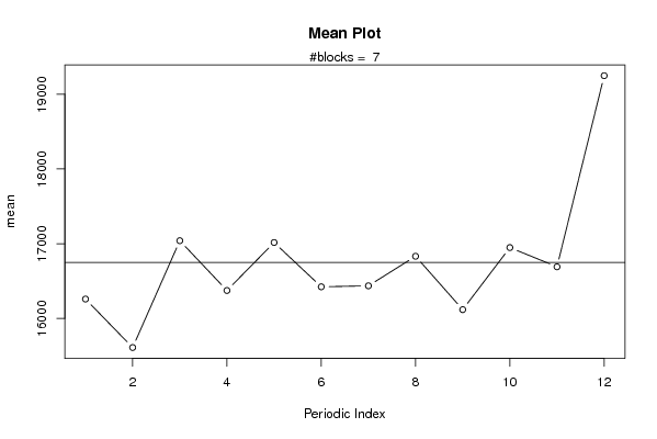
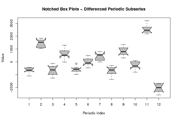
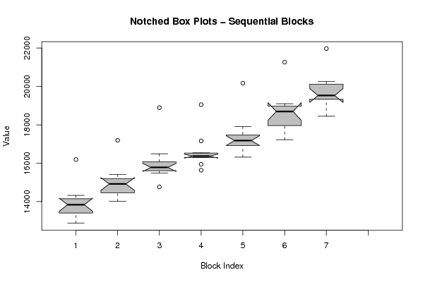
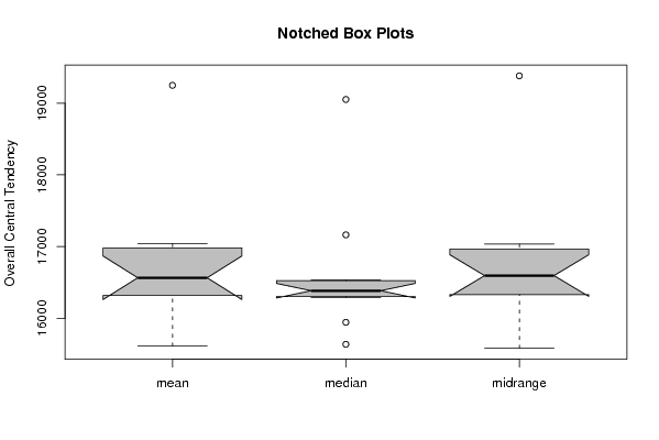
| Title produced by software | Mean Plot | ||||||||||||||||||||
| Date of computation | Mon, 04 Oct 2010 19:03:15 +0000 | ||||||||||||||||||||
| Cite this page as follows | Statistical Computations at FreeStatistics.org, Office for Research Development and Education, URL https://freestatistics.org/blog/index.php?v=date/2010/Oct/04/t12862191293ccxmvrwbprv62v.htm/, Retrieved Sun, 28 Apr 2024 18:14:13 +0000 | ||||||||||||||||||||
| Statistical Computations at FreeStatistics.org, Office for Research Development and Education, URL https://freestatistics.org/blog/index.php?pk=80996, Retrieved Sun, 28 Apr 2024 18:14:13 +0000 | |||||||||||||||||||||
| QR Codes: | |||||||||||||||||||||
|
| |||||||||||||||||||||
| Original text written by user: | |||||||||||||||||||||
| IsPrivate? | No (this computation is public) | ||||||||||||||||||||
| User-defined keywords | |||||||||||||||||||||
| Estimated Impact | 88 | ||||||||||||||||||||
Tree of Dependent Computations | |||||||||||||||||||||
| Family? (F = Feedback message, R = changed R code, M = changed R Module, P = changed Parameters, D = changed Data) | |||||||||||||||||||||
| F [Univariate Data Series] [HPC Retail Sales] [2008-03-02 15:42:48] [74be16979710d4c4e7c6647856088456] - RMPD [Mean Plot] [Time Series Plot] [2010-10-04 19:03:15] [5fd8c857995b7937a45335fd5ccccdde] [Current] | |||||||||||||||||||||
| Feedback Forum | |||||||||||||||||||||
Post a new message | |||||||||||||||||||||
Dataset | |||||||||||||||||||||
| Dataseries X: | |||||||||||||||||||||
13328 12873 14000 13477 14237 13674 13529 14058 12975 14326 14008 16193 14483 14011 15057 14884 15414 14440 14900 15074 14442 15307 14938 17193 15528 14765 15838 15723 16150 15486 15986 15983 15692 16490 15686 18897 16316 15636 17163 16534 16518 16375 16290 16352 15943 16362 16393 19051 16747 16320 17910 16961 17480 17049 16879 17473 16998 17307 17418 20169 17871 17226 19062 17804 19100 18522 18060 18869 18127 18871 18890 21263 19547 18450 20254 19240 20216 19420 19415 20018 18652 19978 19509 21971 | |||||||||||||||||||||
Tables (Output of Computation) | |||||||||||||||||||||
| |||||||||||||||||||||
Figures (Output of Computation) | |||||||||||||||||||||
Input Parameters & R Code | |||||||||||||||||||||
| Parameters (Session): | |||||||||||||||||||||
| par1 = 2000 ; par2 = grey ; par3 = FALSE ; par4 = Unknown ; | |||||||||||||||||||||
| Parameters (R input): | |||||||||||||||||||||
| par1 = 12 ; | |||||||||||||||||||||
| R code (references can be found in the software module): | |||||||||||||||||||||
par1 <- as.numeric(par1) | |||||||||||||||||||||