Repository of Reproducible Computations

Free Statistics

of Irreproducible Research!

Author's title

Author

*The author of this computation has been verified*

R Software Module

rwasp_histogram.wasp

Title produced by software

Histogram

Date of computation

Mon, 04 Oct 2010 16:37:20 +0000

Cite this page as follows

Statistical Computations at FreeStatistics.org, Office for Research Development and Education, URL https://freestatistics.org/blog/index.php?v=date/2010/Oct/04/t1286210180rbcdwopsek4p5kr.htm/, Retrieved Sun, 28 Apr 2024 13:35:11 +0000

Statistical Computations at FreeStatistics.org, Office for Research Development and Education, URL https://freestatistics.org/blog/index.php?pk=80649, Retrieved Sun, 28 Apr 2024 13:35:11 +0000

QR Codes:

Paste this QR Code to cite your computation.

Original text written by user:

IsPrivate?

No (this computation is public)

User-defined keywords

Estimated Impact

121

Family? (F = Feedback message, R = changed R code, M = changed R Module, P = changed Parameters, D = changed Data)

-     [Histogram] [Bad example of Hi...] [2010-09-25 09:28:23] [b98453cac15ba1066b407e146608df68]
F   PD    [Histogram] [ws1 task 3] [2010-10-04 16:37:20] [67e3c2d70de1dbb070b545ca6c893d5e] [Current]

Feedback Forum

2010-10-08 07:51:21 [2367ef1b461dcf270178cda4b96c6ab3] [reply] 
Oefening 3, 
 
Hier heb je wederom de juiste data gebruikt, enkel had je de 'number of bins' moeten veranderen in 30 zo krijg je een nog betere weergave van de histogram. 
wat jij echter hebt gedaan is niet verkeerd, enkele een conclusie ontbreekt. 
 
de normale tijd dat een student nodig heeft om een enquête in te vullen is ongeveer 250 seconden. 
 
2010-10-20 01:11:40 [Naoual Ahidar] [reply] 
De student had de bins beter moeten veranderen om een duidelijker beeld te krijgen. Er ontbreekt een antwoordzin: de normale tijd die een student nodig heeft om een enquête in te vullen is 250 seconden. 

Post a new message

Dataseries X:

Download CSV

Histogram

Boxplots

Summary of computational transaction
Raw Input	view raw input (R code)
Raw Output	view raw output of R engine
Computing time	1 seconds
R Server	'Sir Ronald Aylmer Fisher' @ 193.190.124.24

\begin{tabular}{lllllllll}
\hline
Summary of computational transaction \tabularnewline
Raw Input & view raw input (R code)  \tabularnewline
Raw Output & view raw output of R engine  \tabularnewline
Computing time & 1 seconds \tabularnewline
R Server & 'Sir Ronald Aylmer Fisher' @ 193.190.124.24 \tabularnewline
\hline
\end{tabular}
%Source: https://freestatistics.org/blog/index.php?pk=80649&T=0

[TABLE]
[ROW][C]Summary of computational transaction[/C][/ROW]
[ROW][C]Raw Input[/C][C]view raw input (R code) [/C][/ROW]
[ROW][C]Raw Output[/C][C]view raw output of R engine [/C][/ROW]
[ROW][C]Computing time[/C][C]1 seconds[/C][/ROW]
[ROW][C]R Server[/C][C]'Sir Ronald Aylmer Fisher' @ 193.190.124.24[/C][/ROW]
[/TABLE]
Source: https://freestatistics.org/blog/index.php?pk=80649&T=0

Globally Unique Identifier (entire table): ba.freestatistics.org/blog/index.php?pk=80649&T=0

As an alternative you can also use a QR Code:

The GUIDs for individual cells are displayed in the table below:

Summary of computational transaction
Raw Input	view raw input (R code)
Raw Output	view raw output of R engine
Computing time	1 seconds
R Server	'Sir Ronald Aylmer Fisher' @ 193.190.124.24

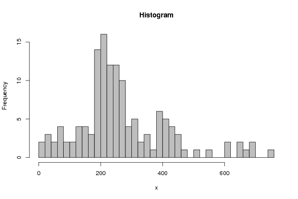
Frequency Table (Histogram)
Bins	Midpoint	Abs. Frequency	Rel. Frequency	Cumul. Rel. Freq.	Density
[0,20[	10	2	0.014925	0.014925	0.000746
[20,40[	30	3	0.022388	0.037313	0.001119
[40,60[	50	2	0.014925	0.052239	0.000746
[60,80[	70	4	0.029851	0.08209	0.001493
[80,100[	90	2	0.014925	0.097015	0.000746
[100,120[	110	2	0.014925	0.11194	0.000746
[120,140[	130	4	0.029851	0.141791	0.001493
[140,160[	150	4	0.029851	0.171642	0.001493
[160,180[	170	3	0.022388	0.19403	0.001119
[180,200[	190	14	0.104478	0.298507	0.005224
[200,220[	210	16	0.119403	0.41791	0.00597
[220,240[	230	12	0.089552	0.507463	0.004478
[240,260[	250	12	0.089552	0.597015	0.004478
[260,280[	270	10	0.074627	0.671642	0.003731
[280,300[	290	4	0.029851	0.701493	0.001493
[300,320[	310	5	0.037313	0.738806	0.001866
[320,340[	330	2	0.014925	0.753731	0.000746
[340,360[	350	3	0.022388	0.776119	0.001119
[360,380[	370	1	0.007463	0.783582	0.000373
[380,400[	390	6	0.044776	0.828358	0.002239
[400,420[	410	5	0.037313	0.865672	0.001866
[420,440[	430	4	0.029851	0.895522	0.001493
[440,460[	450	3	0.022388	0.91791	0.001119
[460,480[	470	1	0.007463	0.925373	0.000373
[480,500[	490	0	0	0.925373	0
[500,520[	510	1	0.007463	0.932836	0.000373
[520,540[	530	0	0	0.932836	0
[540,560[	550	1	0.007463	0.940299	0.000373
[560,580[	570	0	0	0.940299	0
[580,600[	590	0	0	0.940299	0
[600,620[	610	2	0.014925	0.955224	0.000746
[620,640[	630	0	0	0.955224	0
[640,660[	650	2	0.014925	0.970149	0.000746
[660,680[	670	1	0.007463	0.977612	0.000373
[680,700[	690	2	0.014925	0.992537	0.000746
[700,720[	710	0	0	0.992537	0
[720,740[	730	0	0	0.992537	0
[740,760]	750	1	0.007463	1	0.000373

\begin{tabular}{lllllllll}
\hline
Frequency Table (Histogram) \tabularnewline
Bins & Midpoint & Abs. Frequency & Rel. Frequency & Cumul. Rel. Freq. & Density \tabularnewline
[0,20[ & 10 & 2 & 0.014925 & 0.014925 & 0.000746 \tabularnewline
[20,40[ & 30 & 3 & 0.022388 & 0.037313 & 0.001119 \tabularnewline
[40,60[ & 50 & 2 & 0.014925 & 0.052239 & 0.000746 \tabularnewline
[60,80[ & 70 & 4 & 0.029851 & 0.08209 & 0.001493 \tabularnewline
[80,100[ & 90 & 2 & 0.014925 & 0.097015 & 0.000746 \tabularnewline
[100,120[ & 110 & 2 & 0.014925 & 0.11194 & 0.000746 \tabularnewline
[120,140[ & 130 & 4 & 0.029851 & 0.141791 & 0.001493 \tabularnewline
[140,160[ & 150 & 4 & 0.029851 & 0.171642 & 0.001493 \tabularnewline
[160,180[ & 170 & 3 & 0.022388 & 0.19403 & 0.001119 \tabularnewline
[180,200[ & 190 & 14 & 0.104478 & 0.298507 & 0.005224 \tabularnewline
[200,220[ & 210 & 16 & 0.119403 & 0.41791 & 0.00597 \tabularnewline
[220,240[ & 230 & 12 & 0.089552 & 0.507463 & 0.004478 \tabularnewline
[240,260[ & 250 & 12 & 0.089552 & 0.597015 & 0.004478 \tabularnewline
[260,280[ & 270 & 10 & 0.074627 & 0.671642 & 0.003731 \tabularnewline
[280,300[ & 290 & 4 & 0.029851 & 0.701493 & 0.001493 \tabularnewline
[300,320[ & 310 & 5 & 0.037313 & 0.738806 & 0.001866 \tabularnewline
[320,340[ & 330 & 2 & 0.014925 & 0.753731 & 0.000746 \tabularnewline
[340,360[ & 350 & 3 & 0.022388 & 0.776119 & 0.001119 \tabularnewline
[360,380[ & 370 & 1 & 0.007463 & 0.783582 & 0.000373 \tabularnewline
[380,400[ & 390 & 6 & 0.044776 & 0.828358 & 0.002239 \tabularnewline
[400,420[ & 410 & 5 & 0.037313 & 0.865672 & 0.001866 \tabularnewline
[420,440[ & 430 & 4 & 0.029851 & 0.895522 & 0.001493 \tabularnewline
[440,460[ & 450 & 3 & 0.022388 & 0.91791 & 0.001119 \tabularnewline
[460,480[ & 470 & 1 & 0.007463 & 0.925373 & 0.000373 \tabularnewline
[480,500[ & 490 & 0 & 0 & 0.925373 & 0 \tabularnewline
[500,520[ & 510 & 1 & 0.007463 & 0.932836 & 0.000373 \tabularnewline
[520,540[ & 530 & 0 & 0 & 0.932836 & 0 \tabularnewline
[540,560[ & 550 & 1 & 0.007463 & 0.940299 & 0.000373 \tabularnewline
[560,580[ & 570 & 0 & 0 & 0.940299 & 0 \tabularnewline
[580,600[ & 590 & 0 & 0 & 0.940299 & 0 \tabularnewline
[600,620[ & 610 & 2 & 0.014925 & 0.955224 & 0.000746 \tabularnewline
[620,640[ & 630 & 0 & 0 & 0.955224 & 0 \tabularnewline
[640,660[ & 650 & 2 & 0.014925 & 0.970149 & 0.000746 \tabularnewline
[660,680[ & 670 & 1 & 0.007463 & 0.977612 & 0.000373 \tabularnewline
[680,700[ & 690 & 2 & 0.014925 & 0.992537 & 0.000746 \tabularnewline
[700,720[ & 710 & 0 & 0 & 0.992537 & 0 \tabularnewline
[720,740[ & 730 & 0 & 0 & 0.992537 & 0 \tabularnewline
[740,760] & 750 & 1 & 0.007463 & 1 & 0.000373 \tabularnewline
\hline
\end{tabular}
%Source: https://freestatistics.org/blog/index.php?pk=80649&T=1

[TABLE]
[ROW][C]Frequency Table (Histogram)[/C][/ROW]
[ROW][C]Bins[/C][C]Midpoint[/C][C]Abs. Frequency[/C][C]Rel. Frequency[/C][C]Cumul. Rel. Freq.[/C][C]Density[/C][/ROW]
[ROW][C][0,20[[/C][C]10[/C][C]2[/C][C]0.014925[/C][C]0.014925[/C][C]0.000746[/C][/ROW]
[ROW][C][20,40[[/C][C]30[/C][C]3[/C][C]0.022388[/C][C]0.037313[/C][C]0.001119[/C][/ROW]
[ROW][C][40,60[[/C][C]50[/C][C]2[/C][C]0.014925[/C][C]0.052239[/C][C]0.000746[/C][/ROW]
[ROW][C][60,80[[/C][C]70[/C][C]4[/C][C]0.029851[/C][C]0.08209[/C][C]0.001493[/C][/ROW]
[ROW][C][80,100[[/C][C]90[/C][C]2[/C][C]0.014925[/C][C]0.097015[/C][C]0.000746[/C][/ROW]
[ROW][C][100,120[[/C][C]110[/C][C]2[/C][C]0.014925[/C][C]0.11194[/C][C]0.000746[/C][/ROW]
[ROW][C][120,140[[/C][C]130[/C][C]4[/C][C]0.029851[/C][C]0.141791[/C][C]0.001493[/C][/ROW]
[ROW][C][140,160[[/C][C]150[/C][C]4[/C][C]0.029851[/C][C]0.171642[/C][C]0.001493[/C][/ROW]
[ROW][C][160,180[[/C][C]170[/C][C]3[/C][C]0.022388[/C][C]0.19403[/C][C]0.001119[/C][/ROW]
[ROW][C][180,200[[/C][C]190[/C][C]14[/C][C]0.104478[/C][C]0.298507[/C][C]0.005224[/C][/ROW]
[ROW][C][200,220[[/C][C]210[/C][C]16[/C][C]0.119403[/C][C]0.41791[/C][C]0.00597[/C][/ROW]
[ROW][C][220,240[[/C][C]230[/C][C]12[/C][C]0.089552[/C][C]0.507463[/C][C]0.004478[/C][/ROW]
[ROW][C][240,260[[/C][C]250[/C][C]12[/C][C]0.089552[/C][C]0.597015[/C][C]0.004478[/C][/ROW]
[ROW][C][260,280[[/C][C]270[/C][C]10[/C][C]0.074627[/C][C]0.671642[/C][C]0.003731[/C][/ROW]
[ROW][C][280,300[[/C][C]290[/C][C]4[/C][C]0.029851[/C][C]0.701493[/C][C]0.001493[/C][/ROW]
[ROW][C][300,320[[/C][C]310[/C][C]5[/C][C]0.037313[/C][C]0.738806[/C][C]0.001866[/C][/ROW]
[ROW][C][320,340[[/C][C]330[/C][C]2[/C][C]0.014925[/C][C]0.753731[/C][C]0.000746[/C][/ROW]
[ROW][C][340,360[[/C][C]350[/C][C]3[/C][C]0.022388[/C][C]0.776119[/C][C]0.001119[/C][/ROW]
[ROW][C][360,380[[/C][C]370[/C][C]1[/C][C]0.007463[/C][C]0.783582[/C][C]0.000373[/C][/ROW]
[ROW][C][380,400[[/C][C]390[/C][C]6[/C][C]0.044776[/C][C]0.828358[/C][C]0.002239[/C][/ROW]
[ROW][C][400,420[[/C][C]410[/C][C]5[/C][C]0.037313[/C][C]0.865672[/C][C]0.001866[/C][/ROW]
[ROW][C][420,440[[/C][C]430[/C][C]4[/C][C]0.029851[/C][C]0.895522[/C][C]0.001493[/C][/ROW]
[ROW][C][440,460[[/C][C]450[/C][C]3[/C][C]0.022388[/C][C]0.91791[/C][C]0.001119[/C][/ROW]
[ROW][C][460,480[[/C][C]470[/C][C]1[/C][C]0.007463[/C][C]0.925373[/C][C]0.000373[/C][/ROW]
[ROW][C][480,500[[/C][C]490[/C][C]0[/C][C]0[/C][C]0.925373[/C][C]0[/C][/ROW]
[ROW][C][500,520[[/C][C]510[/C][C]1[/C][C]0.007463[/C][C]0.932836[/C][C]0.000373[/C][/ROW]
[ROW][C][520,540[[/C][C]530[/C][C]0[/C][C]0[/C][C]0.932836[/C][C]0[/C][/ROW]
[ROW][C][540,560[[/C][C]550[/C][C]1[/C][C]0.007463[/C][C]0.940299[/C][C]0.000373[/C][/ROW]
[ROW][C][560,580[[/C][C]570[/C][C]0[/C][C]0[/C][C]0.940299[/C][C]0[/C][/ROW]
[ROW][C][580,600[[/C][C]590[/C][C]0[/C][C]0[/C][C]0.940299[/C][C]0[/C][/ROW]
[ROW][C][600,620[[/C][C]610[/C][C]2[/C][C]0.014925[/C][C]0.955224[/C][C]0.000746[/C][/ROW]
[ROW][C][620,640[[/C][C]630[/C][C]0[/C][C]0[/C][C]0.955224[/C][C]0[/C][/ROW]
[ROW][C][640,660[[/C][C]650[/C][C]2[/C][C]0.014925[/C][C]0.970149[/C][C]0.000746[/C][/ROW]
[ROW][C][660,680[[/C][C]670[/C][C]1[/C][C]0.007463[/C][C]0.977612[/C][C]0.000373[/C][/ROW]
[ROW][C][680,700[[/C][C]690[/C][C]2[/C][C]0.014925[/C][C]0.992537[/C][C]0.000746[/C][/ROW]
[ROW][C][700,720[[/C][C]710[/C][C]0[/C][C]0[/C][C]0.992537[/C][C]0[/C][/ROW]
[ROW][C][720,740[[/C][C]730[/C][C]0[/C][C]0[/C][C]0.992537[/C][C]0[/C][/ROW]
[ROW][C][740,760][/C][C]750[/C][C]1[/C][C]0.007463[/C][C]1[/C][C]0.000373[/C][/ROW]
[/TABLE]
Source: https://freestatistics.org/blog/index.php?pk=80649&T=1

Globally Unique Identifier (entire table): ba.freestatistics.org/blog/index.php?pk=80649&T=1

As an alternative you can also use a QR Code:

The GUIDs for individual cells are displayed in the table below:

Frequency Table (Histogram)
Bins	Midpoint	Abs. Frequency	Rel. Frequency	Cumul. Rel. Freq.	Density
[0,20[	10	2	0.014925	0.014925	0.000746
[20,40[	30	3	0.022388	0.037313	0.001119
[40,60[	50	2	0.014925	0.052239	0.000746
[60,80[	70	4	0.029851	0.08209	0.001493
[80,100[	90	2	0.014925	0.097015	0.000746
[100,120[	110	2	0.014925	0.11194	0.000746
[120,140[	130	4	0.029851	0.141791	0.001493
[140,160[	150	4	0.029851	0.171642	0.001493
[160,180[	170	3	0.022388	0.19403	0.001119
[180,200[	190	14	0.104478	0.298507	0.005224
[200,220[	210	16	0.119403	0.41791	0.00597
[220,240[	230	12	0.089552	0.507463	0.004478
[240,260[	250	12	0.089552	0.597015	0.004478
[260,280[	270	10	0.074627	0.671642	0.003731
[280,300[	290	4	0.029851	0.701493	0.001493
[300,320[	310	5	0.037313	0.738806	0.001866
[320,340[	330	2	0.014925	0.753731	0.000746
[340,360[	350	3	0.022388	0.776119	0.001119
[360,380[	370	1	0.007463	0.783582	0.000373
[380,400[	390	6	0.044776	0.828358	0.002239
[400,420[	410	5	0.037313	0.865672	0.001866
[420,440[	430	4	0.029851	0.895522	0.001493
[440,460[	450	3	0.022388	0.91791	0.001119
[460,480[	470	1	0.007463	0.925373	0.000373
[480,500[	490	0	0	0.925373	0
[500,520[	510	1	0.007463	0.932836	0.000373
[520,540[	530	0	0	0.932836	0
[540,560[	550	1	0.007463	0.940299	0.000373
[560,580[	570	0	0	0.940299	0
[580,600[	590	0	0	0.940299	0
[600,620[	610	2	0.014925	0.955224	0.000746
[620,640[	630	0	0	0.955224	0
[640,660[	650	2	0.014925	0.970149	0.000746
[660,680[	670	1	0.007463	0.977612	0.000373
[680,700[	690	2	0.014925	0.992537	0.000746
[700,720[	710	0	0	0.992537	0
[720,740[	730	0	0	0.992537	0
[740,760]	750	1	0.007463	1	0.000373

Figure 1

PNG link

Postscript link

PDF link

Parameters (Session):

par1 = 30 ; par2 = grey ; par3 = FALSE ; par4 = Unknown ;

Parameters (R input):

par1 = 30 ; par2 = grey ; par3 = FALSE ; par4 = Unknown ;

R code (references can be found in the software module):

par1 <- as.numeric(par1)
if (par3 == 'TRUE') par3 <- TRUE
if (par3 == 'FALSE') par3 <- FALSE
if (par4 == 'Unknown') par1 <- as.numeric(par1)
if (par4 == 'Interval/Ratio') par1 <- as.numeric(par1)
if (par4 == '3-point Likert') par1 <- c(1:3 - 0.5, 3.5)
if (par4 == '4-point Likert') par1 <- c(1:4 - 0.5, 4.5)
if (par4 == '5-point Likert') par1 <- c(1:5 - 0.5, 5.5)
if (par4 == '6-point Likert') par1 <- c(1:6 - 0.5, 6.5)
if (par4 == '7-point Likert') par1 <- c(1:7 - 0.5, 7.5)
if (par4 == '8-point Likert') par1 <- c(1:8 - 0.5, 8.5)
if (par4 == '9-point Likert') par1 <- c(1:9 - 0.5, 9.5)
if (par4 == '10-point Likert') par1 <- c(1:10 - 0.5, 10.5)
bitmap(file='test1.png')
if(is.numeric(x[1])) {
if (is.na(par1)) {
myhist<-hist(x,col=par2,main=main,xlab=xlab,right=par3)
} else {
if (par1 < 0) par1 <- 3
if (par1 > 50) par1 <- 50
myhist<-hist(x,breaks=par1,col=par2,main=main,xlab=xlab,right=par3)
}
} else {
plot(mytab <- table(x),col=par2,main='Frequency Plot',xlab=xlab,ylab='Absolute Frequency')
}
dev.off()
if(is.numeric(x[1])) {
myhist
n <- length(x)
load(file='createtable')
a<-table.start()
a<-table.row.start(a)
a<-table.element(a,hyperlink('histogram.htm','Frequency Table (Histogram)',''),6,TRUE)
a<-table.row.end(a)
a<-table.row.start(a)
a<-table.element(a,'Bins',header=TRUE)
a<-table.element(a,'Midpoint',header=TRUE)
a<-table.element(a,'Abs. Frequency',header=TRUE)
a<-table.element(a,'Rel. Frequency',header=TRUE)
a<-table.element(a,'Cumul. Rel. Freq.',header=TRUE)
a<-table.element(a,'Density',header=TRUE)
a<-table.row.end(a)
crf <- 0
if (par3 == FALSE) mybracket <- '[' else mybracket <- ']'
mynumrows <- (length(myhist$breaks)-1)
for (i in 1:mynumrows) {
a<-table.row.start(a)
if (i == 1)
dum <- paste('[',myhist$breaks[i],sep='')
else
dum <- paste(mybracket,myhist$breaks[i],sep='')
dum <- paste(dum,myhist$breaks[i+1],sep=',')
if (i==mynumrows)
dum <- paste(dum,']',sep='')
else
dum <- paste(dum,mybracket,sep='')
a<-table.element(a,dum,header=TRUE)
a<-table.element(a,myhist$mids[i])
a<-table.element(a,myhist$counts[i])
rf <- myhist$counts[i]/n
crf <- crf + rf
a<-table.element(a,round(rf,6))
a<-table.element(a,round(crf,6))
a<-table.element(a,round(myhist$density[i],6))
a<-table.row.end(a)
}
a<-table.end(a)
table.save(a,file='mytable.tab')
} else {
mytab
reltab <- mytab / sum(mytab)
n <- length(mytab)
load(file='createtable')
a<-table.start()
a<-table.row.start(a)
a<-table.element(a,'Frequency Table (Categorical Data)',3,TRUE)
a<-table.row.end(a)
a<-table.row.start(a)
a<-table.element(a,'Category',header=TRUE)
a<-table.element(a,'Abs. Frequency',header=TRUE)
a<-table.element(a,'Rel. Frequency',header=TRUE)
a<-table.row.end(a)
for (i in 1:n) {
a<-table.row.start(a)
a<-table.element(a,labels(mytab)$x[i],header=TRUE)
a<-table.element(a,mytab[i])
a<-table.element(a,round(reltab[i],4))
a<-table.row.end(a)
}
a<-table.end(a)
table.save(a,file='mytable1.tab')
}

Free Statistics

Description of Statistical Computation

Tree of Dependent Computations

Dataset

Tables (Output of Computation)

Figures (Output of Computation)

Input Parameters & R Code