Free Statistics
of Irreproducible Research!
Description of Statistical Computation | |||||||||||||||||||||||||||||||||||||||||||||||||||||||||||||
|---|---|---|---|---|---|---|---|---|---|---|---|---|---|---|---|---|---|---|---|---|---|---|---|---|---|---|---|---|---|---|---|---|---|---|---|---|---|---|---|---|---|---|---|---|---|---|---|---|---|---|---|---|---|---|---|---|---|---|---|---|---|
| Author's title | |||||||||||||||||||||||||||||||||||||||||||||||||||||||||||||
| Author | *The author of this computation has been verified* | ||||||||||||||||||||||||||||||||||||||||||||||||||||||||||||
| R Software Module | rwasp_linear_regression.wasp | ||||||||||||||||||||||||||||||||||||||||||||||||||||||||||||
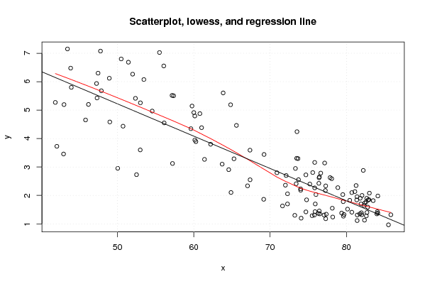
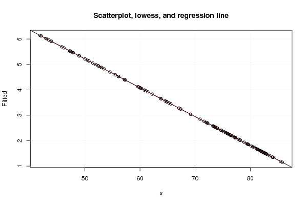
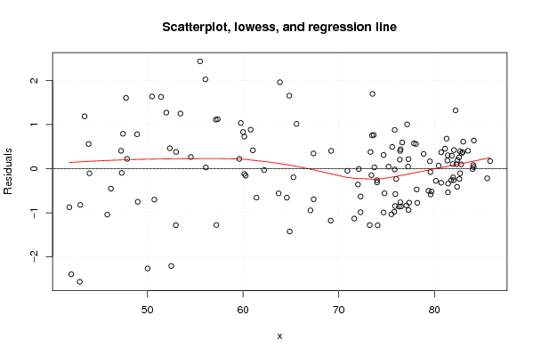
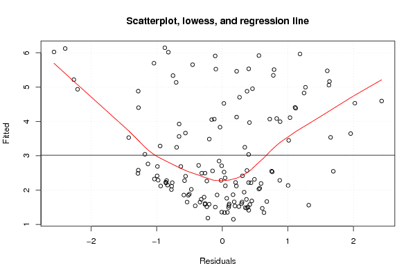
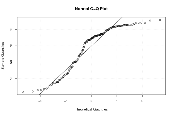
| Title produced by software | Linear Regression Graphical Model Validation | ||||||||||||||||||||||||||||||||||||||||||||||||||||||||||||
| Date of computation | Thu, 25 Nov 2010 09:23:05 +0000 | ||||||||||||||||||||||||||||||||||||||||||||||||||||||||||||
| Cite this page as follows | Statistical Computations at FreeStatistics.org, Office for Research Development and Education, URL https://freestatistics.org/blog/index.php?v=date/2010/Nov/25/t1290676898n5fu9rzicgfbu8m.htm/, Retrieved Sat, 12 Jul 2025 03:25:11 +0000 | ||||||||||||||||||||||||||||||||||||||||||||||||||||||||||||
| Statistical Computations at FreeStatistics.org, Office for Research Development and Education, URL https://freestatistics.org/blog/index.php?pk=100651, Retrieved Sat, 12 Jul 2025 03:25:11 +0000 | |||||||||||||||||||||||||||||||||||||||||||||||||||||||||||||
| QR Codes: | |||||||||||||||||||||||||||||||||||||||||||||||||||||||||||||
|
| |||||||||||||||||||||||||||||||||||||||||||||||||||||||||||||
| Original text written by user: | |||||||||||||||||||||||||||||||||||||||||||||||||||||||||||||
| IsPrivate? | No (this computation is public) | ||||||||||||||||||||||||||||||||||||||||||||||||||||||||||||
| User-defined keywords | |||||||||||||||||||||||||||||||||||||||||||||||||||||||||||||
| Estimated Impact | 258 | ||||||||||||||||||||||||||||||||||||||||||||||||||||||||||||
Tree of Dependent Computations | |||||||||||||||||||||||||||||||||||||||||||||||||||||||||||||
| Family? (F = Feedback message, R = changed R code, M = changed R Module, P = changed Parameters, D = changed Data) | |||||||||||||||||||||||||||||||||||||||||||||||||||||||||||||
| - [Linear Regression Graphical Model Validation] [Colombia Coffee -...] [2008-02-26 10:22:06] [74be16979710d4c4e7c6647856088456] - M D [Linear Regression Graphical Model Validation] [] [2010-11-25 09:23:05] [b91d9cfbf8712a09013bf3c2e3081c55] [Current] - D [Linear Regression Graphical Model Validation] [] [2010-11-25 18:35:56] [234dae34fc2a42f724a2786a39cb083b] - D [Linear Regression Graphical Model Validation] [] [2010-11-25 21:09:47] [afd301b68d203992295e6972aed62880] - D [Linear Regression Graphical Model Validation] [Paper - Autocorre...] [2010-11-30 21:57:38] [8677c3f87cec9201607d40be65aa9670] - D [Linear Regression Graphical Model Validation] [Paper - Autocorre...] [2010-11-30 22:15:19] [8677c3f87cec9201607d40be65aa9670] | |||||||||||||||||||||||||||||||||||||||||||||||||||||||||||||
| Feedback Forum | |||||||||||||||||||||||||||||||||||||||||||||||||||||||||||||
Post a new message | |||||||||||||||||||||||||||||||||||||||||||||||||||||||||||||
Dataset | |||||||||||||||||||||||||||||||||||||||||||||||||||||||||||||
| Dataseries X: | |||||||||||||||||||||||||||||||||||||||||||||||||||||||||||||
83,5 82,68 82,4 82,782566 81,384 79,67 80,43 82,83 84,11 82 81,95 77,35 83 81,8 82,2 83,98 85,81 82,36 82,3 77,238835 81,9 82,035 82,66 79,6 81,75 78,2 81,415 84,1 82,94 84,04 74 81,345 80,7 43,452 79,574 73,412 43,958 78,868 77,28 64,576 75,5 57,354 67,04 67,358 77,28 50,036 75,84 76,3 53,46 50,492 61,402 50,732 45,822 51,988 76,38 56,118 47,46 81,104 48,998 79,37 80,138 75,2 77,856 73,312 74,684 52,356 59,768 78,14 70,892 57,212 60,134 74,686 60,138 73,516 57,154 47,778 62,204 73,472 85,5 72,278 61,024 72 54,55 69,158 72,1 65,264 76,5 73,988 42,94 46,2 76,63 77,06 76,434 60,796 47,886 76,452 56,066 80,7 65,586 75,91 72,274 43 64,876 52,984 63,716 75,58 55,508 47,328 77,142 78,064 60,274 73,714 73,648 82,56 75,8 73,23 47,262 64,822 75,88 43,87 82,6 48,934 52,5 59,622 75,838 81,4 69,204 53,002 74,774 60,004 71,62 76 67,372 51,432 74,06 81,258 79,52 76,41 63,848 41,86 42,062 | |||||||||||||||||||||||||||||||||||||||||||||||||||||||||||||
| Dataseries Y: | |||||||||||||||||||||||||||||||||||||||||||||||||||||||||||||
1,817 1,4 1,7324337 1,59 1,9552 1,33 1,83 1,84 1,98 1,32 1,39 1,34 2,08 1,9 2,88 1,35 1,32 1,13 1,65 2,171569 1,7 2 1,9 1,27 1,35 1,24 1,31 1,38 1,85 1,43 2,18 1,84 2,1 7,151 1,78 2,4116 5,8 2,2732 2,3348 2,9056 1,287 5,5052 2,3368 3,5916 1,18 2,9528 2,265 1,37 6,0754 6,8 3,2674 4,4346 4,654 6,2644 2,425 4,5502 6,3 2,1354 4,5832 1,38 1,518 2,4 2,6258 2,9476 2,723 5,414 5,1436 1,55 2,7976 3,1232 4,7934 1,4212 3,9466 4,2416 5,5176 7,0752 3,8 3,3053333 0,966 2,0568 4,3828 2,36 4,9672 1,8634 2,7 3,2878 1,35 2,231 3,457 5,2 2,7852 1,31 1,453 4,8764 5,6808 2,6524 6,5538 1,41 4,4626 1,7 1,7 5,1942 2,1034 3,6 3,1 2,804 7,02575 5,4266 3,1396 2,5888 3,8918 2,553 3,2952 1,7728 1,31 1,3 5,9356 5,1885714 1,43 6,4768 1,28 6,1208 2,73 4,3464 3,1606 1,115 3,4402 5,2576 1,845 4,9142 1,63 2,03 2,5502 6,685 1,2 2,347 2,03 2,62 5,6052 5,2704 3,7274286 | |||||||||||||||||||||||||||||||||||||||||||||||||||||||||||||
Tables (Output of Computation) | |||||||||||||||||||||||||||||||||||||||||||||||||||||||||||||
| |||||||||||||||||||||||||||||||||||||||||||||||||||||||||||||
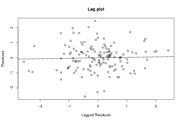
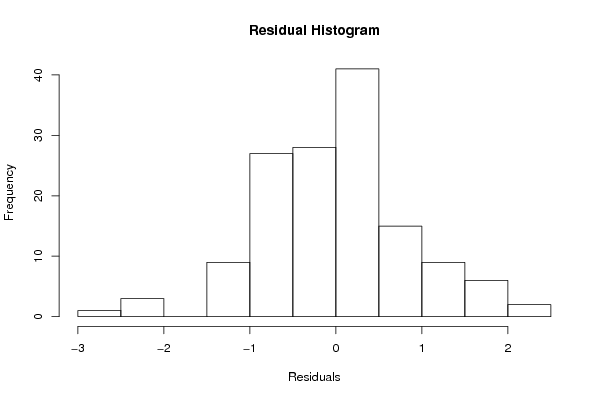
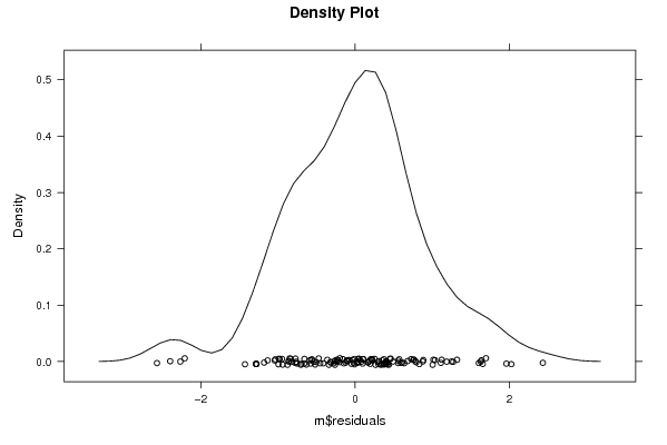
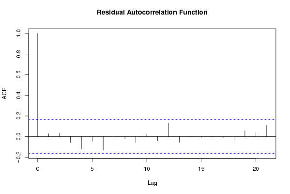
Figures (Output of Computation) | |||||||||||||||||||||||||||||||||||||||||||||||||||||||||||||
Input Parameters & R Code | |||||||||||||||||||||||||||||||||||||||||||||||||||||||||||||
| Parameters (Session): | |||||||||||||||||||||||||||||||||||||||||||||||||||||||||||||
| par1 = 0 ; | |||||||||||||||||||||||||||||||||||||||||||||||||||||||||||||
| Parameters (R input): | |||||||||||||||||||||||||||||||||||||||||||||||||||||||||||||
| par1 = 0 ; | |||||||||||||||||||||||||||||||||||||||||||||||||||||||||||||
| R code (references can be found in the software module): | |||||||||||||||||||||||||||||||||||||||||||||||||||||||||||||
par1 <- as.numeric(par1) | |||||||||||||||||||||||||||||||||||||||||||||||||||||||||||||