Repository of Reproducible Computations

Free Statistics

of Irreproducible Research!

Author's title

Author

*The author of this computation has been verified*

R Software Module

rwasp_autocorrelation.wasp

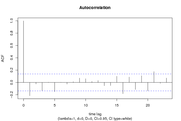
Title produced by software

(Partial) Autocorrelation Function

Date of computation

Tue, 23 Nov 2010 17:55:10 +0000

Cite this page as follows

Statistical Computations at FreeStatistics.org, Office for Research Development and Education, URL https://freestatistics.org/blog/index.php?v=date/2010/Nov/23/t1290534832852m5aih3c9qahh.htm/, Retrieved Wed, 24 Apr 2024 08:23:08 +0000

Statistical Computations at FreeStatistics.org, Office for Research Development and Education, URL https://freestatistics.org/blog/index.php?pk=99508, Retrieved Wed, 24 Apr 2024 08:23:08 +0000

QR Codes:

Paste this QR Code to cite your computation.

Original text written by user:

IsPrivate?

No (this computation is public)

User-defined keywords

Estimated Impact

106

Family? (F = Feedback message, R = changed R code, M = changed R Module, P = changed Parameters, D = changed Data)

-     [Central Tendency] [] [2010-10-20 18:18:38] [b98453cac15ba1066b407e146608df68]
- RMPD    [(Partial) Autocorrelation Function] [GUN autocorrelatie] [2010-11-23 17:55:10] [f76239c595e4d455b3b05a43389f68d5] [Current]

Feedback Forum

Post a new message

Dataseries X:

Download CSV

Histogram

Boxplots

-0.07331526501745
3.2862601528905E-14
3.2862601528905E-14
3.2862601528905E-14
3.2862601528905E-14
3.2862601528905E-14
3.2862601528905E-14
3.2862601528905E-14
0.073315265017433
-0.07331526501745
3.2862601528905E-14
3.2862601528905E-14
3.2862601528905E-14
3.2862601528905E-14
3.2862601528905E-14
3.2862601528905E-14
0.073315265017433
-4.9737991503207E-14
-4.9737991503207E-14
-4.9737991503207E-14
-4.9737991503207E-14
-4.9737991503207E-14
-4.9737991503207E-14
-4.9737991503207E-14
-0.03293710907405
3.5527136788005E-14
3.5527136788005E-14
0.071931219008635
-0.0085349024497958
0.0085349024498416
-0.0085349024497958
4.1744385725906E-14
-0.063396316558758
3.5527136788005E-14
3.5527136788005E-14
3.5527136788005E-14
3.5527136788005E-14
0.071931219008635
0.036848103398004
2.3536728122053E-14
2.3536728122053E-14
-0.067774696162676
4.2632564145606E-14
4.2632564145606E-14
0.036576325306843
-1.5099033134902E-14
-1.5099033134902E-14
-1.5099033134902E-14
-1.5099033134902E-14
-1.5099033134902E-14
-1.5099033134902E-14
-1.5099033134902E-14
0.031198370855885
-0.031198370855877
0.031198370855885
-0.031198370855877
-1.5099033134902E-14
-1.5099033134902E-14
0.031198370855885
-0.031198370855877
-1.5099033134902E-14
0.031198370855885
2.3536728122053E-14
2.3536728122053E-14
2.3536728122053E-14
-0.031198370855877
0.031198370855885
2.3536728122053E-14
2.3536728122053E-14
2.3536728122053E-14
2.3536728122053E-14
-0.031198370855877
-1.5099033134902E-14
-1.5099033134902E-14
-1.5099033134902E-14
0.031198370855885
2.3536728122053E-14
2.3536728122053E-14
2.3536728122053E-14
2.3536728122053E-14
2.3536728122053E-14
2.3536728122053E-14
2.3536728122053E-14
2.3536728122053E-14
-0.031198370855877
0.031198370855885
-0.031198370855877
-1.5099033134902E-14
-1.5099033134902E-14
0.031198370855885
2.3536728122053E-14
-0.031198370855877
0.031198370855885
2.3536728122053E-14
-0.031198370855877
-1.5099033134902E-14
0.031198370855885
2.3536728122053E-14
2.3536728122053E-14
2.3536728122053E-14
2.3536728122053E-14
2.3536728122053E-14
-0.031198370855877
0.031198370855885
2.3536728122053E-14
2.3536728122053E-14
2.3536728122053E-14
2.3536728122053E-14
2.3536728122053E-14
2.3536728122053E-14
2.3536728122053E-14
2.3536728122053E-14
-0.031198370855877
-1.5099033134902E-14
-1.5099033134902E-14
-1.5099033134902E-14
-1.5099033134902E-14
-1.5099033134902E-14
-1.5099033134902E-14
-1.5099033134902E-14
-1.5099033134902E-14
-1.5099033134902E-14
0.031198370855885
2.3536728122053E-14
2.3536728122053E-14
2.3536728122053E-14
2.3536728122053E-14
-0.031198370855877
-1.5099033134902E-14
-1.5099033134902E-14
-1.5099033134902E-14
-1.5099033134902E-14
0.031198370855885
-0.031198370855877
-1.5099033134902E-14
-1.5099033134902E-14
0.031198370855885
2.3536728122053E-14
2.3536728122053E-14
2.3536728122053E-14
2.3536728122053E-14
2.3536728122053E-14
-0.031198370855877
-1.5099033134902E-14
-1.5099033134902E-14
0.031198370855885
-0.031198370855877
-1.5099033134902E-14
-1.5099033134902E-14
-1.5099033134902E-14
-1.5099033134902E-14
0.031198370855885
-0.045383005847776
0.014184634991941
-1.5099033134902E-14
-1.5099033134902E-14
0.031198370855885
2.3536728122053E-14
2.3536728122053E-14
-0.031198370855877
0.031198370855885
2.3536728122053E-14
2.3536728122053E-14
2.3536728122053E-14
-0.031198370855877
-1.5099033134902E-14
0.031198370855885
-0.031198370855877
-1.5099033134902E-14
-1.5099033134902E-14
0.031198370855885
-0.031198370855877
-1.5099033134902E-14
-1.5099033134902E-14
-1.5099033134902E-14
-1.5099033134902E-14
-1.5099033134902E-14
0.031198370855885
2.3536728122053E-14
-0.031198370855877
-1.5099033134902E-14
-1.5099033134902E-14
0.031198370855885
2.3536728122053E-14
-0.031198370855877
-1.5099033134902E-14
-1.5099033134902E-14
-1.5099033134902E-14
-1.5099033134902E-14
-1.5099033134902E-14
-1.5099033134902E-14
-1.5099033134902E-14
-1.5099033134902E-14
-1.5099033134902E-14
-1.5099033134902E-14
-1.5099033134902E-14
-1.5099033134902E-14
-1.5099033134902E-14
-1.5099033134902E-14
-1.5099033134902E-14

Summary of computational transaction
Raw Input	view raw input (R code)
Raw Output	view raw output of R engine
Computing time	2 seconds
R Server	'Gwilym Jenkins' @ 72.249.127.135

\begin{tabular}{lllllllll}
\hline
Summary of computational transaction \tabularnewline
Raw Input & view raw input (R code)  \tabularnewline
Raw Output & view raw output of R engine  \tabularnewline
Computing time & 2 seconds \tabularnewline
R Server & 'Gwilym Jenkins' @ 72.249.127.135 \tabularnewline
\hline
\end{tabular}
%Source: https://freestatistics.org/blog/index.php?pk=99508&T=0

[TABLE]
[ROW][C]Summary of computational transaction[/C][/ROW]
[ROW][C]Raw Input[/C][C]view raw input (R code) [/C][/ROW]
[ROW][C]Raw Output[/C][C]view raw output of R engine [/C][/ROW]
[ROW][C]Computing time[/C][C]2 seconds[/C][/ROW]
[ROW][C]R Server[/C][C]'Gwilym Jenkins' @ 72.249.127.135[/C][/ROW]
[/TABLE]
Source: https://freestatistics.org/blog/index.php?pk=99508&T=0

Globally Unique Identifier (entire table): ba.freestatistics.org/blog/index.php?pk=99508&T=0

As an alternative you can also use a QR Code:

The GUIDs for individual cells are displayed in the table below:

Summary of computational transaction
Raw Input	view raw input (R code)
Raw Output	view raw output of R engine
Computing time	2 seconds
R Server	'Gwilym Jenkins' @ 72.249.127.135

Autocorrelation Function
Time lag k	ACF(k)	T-STAT	P-value
1	-0.216756	-3.0654	0.001237
2	-0.025398	-0.3592	0.359917
3	-0.135244	-1.9126	0.028612
4	0.003892	0.055	0.47808
5	-0.150414	-2.1272	0.017315
6	0.002705	0.0383	0.484762
7	-0.027228	-0.3851	0.350302
8	0.012275	0.1736	0.43118
9	0.070843	1.0019	0.158809
10	0.061459	0.8692	0.1929
11	0.015978	0.226	0.41073
12	0.032749	0.4631	0.321882
13	-0.054317	-0.7682	0.221648
14	-0.050889	-0.7197	0.236282
15	0.100897	1.4269	0.077585
16	-0.183683	-2.5977	0.005042
17	0.088054	1.2453	0.107245
18	-0.115087	-1.6276	0.052595
19	0.109452	1.5479	0.061615
20	-0.137018	-1.9377	0.027032
21	0.177208	2.5061	0.006502
22	-0.014559	-0.2059	0.418543
23	0.071701	1.014	0.155904

\begin{tabular}{lllllllll}
\hline
Autocorrelation Function \tabularnewline
Time lag k & ACF(k) & T-STAT & P-value \tabularnewline
1 & -0.216756 & -3.0654 & 0.001237 \tabularnewline
2 & -0.025398 & -0.3592 & 0.359917 \tabularnewline
3 & -0.135244 & -1.9126 & 0.028612 \tabularnewline
4 & 0.003892 & 0.055 & 0.47808 \tabularnewline
5 & -0.150414 & -2.1272 & 0.017315 \tabularnewline
6 & 0.002705 & 0.0383 & 0.484762 \tabularnewline
7 & -0.027228 & -0.3851 & 0.350302 \tabularnewline
8 & 0.012275 & 0.1736 & 0.43118 \tabularnewline
9 & 0.070843 & 1.0019 & 0.158809 \tabularnewline
10 & 0.061459 & 0.8692 & 0.1929 \tabularnewline
11 & 0.015978 & 0.226 & 0.41073 \tabularnewline
12 & 0.032749 & 0.4631 & 0.321882 \tabularnewline
13 & -0.054317 & -0.7682 & 0.221648 \tabularnewline
14 & -0.050889 & -0.7197 & 0.236282 \tabularnewline
15 & 0.100897 & 1.4269 & 0.077585 \tabularnewline
16 & -0.183683 & -2.5977 & 0.005042 \tabularnewline
17 & 0.088054 & 1.2453 & 0.107245 \tabularnewline
18 & -0.115087 & -1.6276 & 0.052595 \tabularnewline
19 & 0.109452 & 1.5479 & 0.061615 \tabularnewline
20 & -0.137018 & -1.9377 & 0.027032 \tabularnewline
21 & 0.177208 & 2.5061 & 0.006502 \tabularnewline
22 & -0.014559 & -0.2059 & 0.418543 \tabularnewline
23 & 0.071701 & 1.014 & 0.155904 \tabularnewline
\hline
\end{tabular}
%Source: https://freestatistics.org/blog/index.php?pk=99508&T=1

[TABLE]
[ROW][C]Autocorrelation Function[/C][/ROW]
[ROW][C]Time lag k[/C][C]ACF(k)[/C][C]T-STAT[/C][C]P-value[/C][/ROW]
[ROW][C]1[/C][C]-0.216756[/C][C]-3.0654[/C][C]0.001237[/C][/ROW]
[ROW][C]2[/C][C]-0.025398[/C][C]-0.3592[/C][C]0.359917[/C][/ROW]
[ROW][C]3[/C][C]-0.135244[/C][C]-1.9126[/C][C]0.028612[/C][/ROW]
[ROW][C]4[/C][C]0.003892[/C][C]0.055[/C][C]0.47808[/C][/ROW]
[ROW][C]5[/C][C]-0.150414[/C][C]-2.1272[/C][C]0.017315[/C][/ROW]
[ROW][C]6[/C][C]0.002705[/C][C]0.0383[/C][C]0.484762[/C][/ROW]
[ROW][C]7[/C][C]-0.027228[/C][C]-0.3851[/C][C]0.350302[/C][/ROW]
[ROW][C]8[/C][C]0.012275[/C][C]0.1736[/C][C]0.43118[/C][/ROW]
[ROW][C]9[/C][C]0.070843[/C][C]1.0019[/C][C]0.158809[/C][/ROW]
[ROW][C]10[/C][C]0.061459[/C][C]0.8692[/C][C]0.1929[/C][/ROW]
[ROW][C]11[/C][C]0.015978[/C][C]0.226[/C][C]0.41073[/C][/ROW]
[ROW][C]12[/C][C]0.032749[/C][C]0.4631[/C][C]0.321882[/C][/ROW]
[ROW][C]13[/C][C]-0.054317[/C][C]-0.7682[/C][C]0.221648[/C][/ROW]
[ROW][C]14[/C][C]-0.050889[/C][C]-0.7197[/C][C]0.236282[/C][/ROW]
[ROW][C]15[/C][C]0.100897[/C][C]1.4269[/C][C]0.077585[/C][/ROW]
[ROW][C]16[/C][C]-0.183683[/C][C]-2.5977[/C][C]0.005042[/C][/ROW]
[ROW][C]17[/C][C]0.088054[/C][C]1.2453[/C][C]0.107245[/C][/ROW]
[ROW][C]18[/C][C]-0.115087[/C][C]-1.6276[/C][C]0.052595[/C][/ROW]
[ROW][C]19[/C][C]0.109452[/C][C]1.5479[/C][C]0.061615[/C][/ROW]
[ROW][C]20[/C][C]-0.137018[/C][C]-1.9377[/C][C]0.027032[/C][/ROW]
[ROW][C]21[/C][C]0.177208[/C][C]2.5061[/C][C]0.006502[/C][/ROW]
[ROW][C]22[/C][C]-0.014559[/C][C]-0.2059[/C][C]0.418543[/C][/ROW]
[ROW][C]23[/C][C]0.071701[/C][C]1.014[/C][C]0.155904[/C][/ROW]
[/TABLE]
Source: https://freestatistics.org/blog/index.php?pk=99508&T=1

Globally Unique Identifier (entire table): ba.freestatistics.org/blog/index.php?pk=99508&T=1

As an alternative you can also use a QR Code:

The GUIDs for individual cells are displayed in the table below:

Autocorrelation Function
Time lag k	ACF(k)	T-STAT	P-value
1	-0.216756	-3.0654	0.001237
2	-0.025398	-0.3592	0.359917
3	-0.135244	-1.9126	0.028612
4	0.003892	0.055	0.47808
5	-0.150414	-2.1272	0.017315
6	0.002705	0.0383	0.484762
7	-0.027228	-0.3851	0.350302
8	0.012275	0.1736	0.43118
9	0.070843	1.0019	0.158809
10	0.061459	0.8692	0.1929
11	0.015978	0.226	0.41073
12	0.032749	0.4631	0.321882
13	-0.054317	-0.7682	0.221648
14	-0.050889	-0.7197	0.236282
15	0.100897	1.4269	0.077585
16	-0.183683	-2.5977	0.005042
17	0.088054	1.2453	0.107245
18	-0.115087	-1.6276	0.052595
19	0.109452	1.5479	0.061615
20	-0.137018	-1.9377	0.027032
21	0.177208	2.5061	0.006502
22	-0.014559	-0.2059	0.418543
23	0.071701	1.014	0.155904

Partial Autocorrelation Function
Time lag k	PACF(k)	T-STAT	P-value
1	-0.216756	-3.0654	0.001237
2	-0.07595	-1.0741	0.142037
3	-0.166361	-2.3527	0.009805
4	-0.07417	-1.0489	0.14774
5	-0.203928	-2.884	0.002178
6	-0.129331	-1.829	0.034443
7	-0.123045	-1.7401	0.041688
8	-0.117166	-1.657	0.049546
9	-0.017028	-0.2408	0.404973
10	0.009527	0.1347	0.446478
11	0.009909	0.1401	0.444346
12	0.053453	0.7559	0.225286
13	-0.012099	-0.1711	0.432155
14	-0.02915	-0.4122	0.340304
15	0.137115	1.9391	0.026948
16	-0.130488	-1.8454	0.03323
17	0.047422	0.6706	0.251611
18	-0.115575	-1.6345	0.051865
19	-0.002282	-0.0323	0.487145
20	-0.149762	-2.118	0.017707
21	0.028852	0.408	0.341847
22	0.010864	0.1536	0.439025
23	0.042219	0.5971	0.275571

\begin{tabular}{lllllllll}
\hline
Partial Autocorrelation Function \tabularnewline
Time lag k & PACF(k) & T-STAT & P-value \tabularnewline
1 & -0.216756 & -3.0654 & 0.001237 \tabularnewline
2 & -0.07595 & -1.0741 & 0.142037 \tabularnewline
3 & -0.166361 & -2.3527 & 0.009805 \tabularnewline
4 & -0.07417 & -1.0489 & 0.14774 \tabularnewline
5 & -0.203928 & -2.884 & 0.002178 \tabularnewline
6 & -0.129331 & -1.829 & 0.034443 \tabularnewline
7 & -0.123045 & -1.7401 & 0.041688 \tabularnewline
8 & -0.117166 & -1.657 & 0.049546 \tabularnewline
9 & -0.017028 & -0.2408 & 0.404973 \tabularnewline
10 & 0.009527 & 0.1347 & 0.446478 \tabularnewline
11 & 0.009909 & 0.1401 & 0.444346 \tabularnewline
12 & 0.053453 & 0.7559 & 0.225286 \tabularnewline
13 & -0.012099 & -0.1711 & 0.432155 \tabularnewline
14 & -0.02915 & -0.4122 & 0.340304 \tabularnewline
15 & 0.137115 & 1.9391 & 0.026948 \tabularnewline
16 & -0.130488 & -1.8454 & 0.03323 \tabularnewline
17 & 0.047422 & 0.6706 & 0.251611 \tabularnewline
18 & -0.115575 & -1.6345 & 0.051865 \tabularnewline
19 & -0.002282 & -0.0323 & 0.487145 \tabularnewline
20 & -0.149762 & -2.118 & 0.017707 \tabularnewline
21 & 0.028852 & 0.408 & 0.341847 \tabularnewline
22 & 0.010864 & 0.1536 & 0.439025 \tabularnewline
23 & 0.042219 & 0.5971 & 0.275571 \tabularnewline
\hline
\end{tabular}
%Source: https://freestatistics.org/blog/index.php?pk=99508&T=2

[TABLE]
[ROW][C]Partial Autocorrelation Function[/C][/ROW]
[ROW][C]Time lag k[/C][C]PACF(k)[/C][C]T-STAT[/C][C]P-value[/C][/ROW]
[ROW][C]1[/C][C]-0.216756[/C][C]-3.0654[/C][C]0.001237[/C][/ROW]
[ROW][C]2[/C][C]-0.07595[/C][C]-1.0741[/C][C]0.142037[/C][/ROW]
[ROW][C]3[/C][C]-0.166361[/C][C]-2.3527[/C][C]0.009805[/C][/ROW]
[ROW][C]4[/C][C]-0.07417[/C][C]-1.0489[/C][C]0.14774[/C][/ROW]
[ROW][C]5[/C][C]-0.203928[/C][C]-2.884[/C][C]0.002178[/C][/ROW]
[ROW][C]6[/C][C]-0.129331[/C][C]-1.829[/C][C]0.034443[/C][/ROW]
[ROW][C]7[/C][C]-0.123045[/C][C]-1.7401[/C][C]0.041688[/C][/ROW]
[ROW][C]8[/C][C]-0.117166[/C][C]-1.657[/C][C]0.049546[/C][/ROW]
[ROW][C]9[/C][C]-0.017028[/C][C]-0.2408[/C][C]0.404973[/C][/ROW]
[ROW][C]10[/C][C]0.009527[/C][C]0.1347[/C][C]0.446478[/C][/ROW]
[ROW][C]11[/C][C]0.009909[/C][C]0.1401[/C][C]0.444346[/C][/ROW]
[ROW][C]12[/C][C]0.053453[/C][C]0.7559[/C][C]0.225286[/C][/ROW]
[ROW][C]13[/C][C]-0.012099[/C][C]-0.1711[/C][C]0.432155[/C][/ROW]
[ROW][C]14[/C][C]-0.02915[/C][C]-0.4122[/C][C]0.340304[/C][/ROW]
[ROW][C]15[/C][C]0.137115[/C][C]1.9391[/C][C]0.026948[/C][/ROW]
[ROW][C]16[/C][C]-0.130488[/C][C]-1.8454[/C][C]0.03323[/C][/ROW]
[ROW][C]17[/C][C]0.047422[/C][C]0.6706[/C][C]0.251611[/C][/ROW]
[ROW][C]18[/C][C]-0.115575[/C][C]-1.6345[/C][C]0.051865[/C][/ROW]
[ROW][C]19[/C][C]-0.002282[/C][C]-0.0323[/C][C]0.487145[/C][/ROW]
[ROW][C]20[/C][C]-0.149762[/C][C]-2.118[/C][C]0.017707[/C][/ROW]
[ROW][C]21[/C][C]0.028852[/C][C]0.408[/C][C]0.341847[/C][/ROW]
[ROW][C]22[/C][C]0.010864[/C][C]0.1536[/C][C]0.439025[/C][/ROW]
[ROW][C]23[/C][C]0.042219[/C][C]0.5971[/C][C]0.275571[/C][/ROW]
[/TABLE]
Source: https://freestatistics.org/blog/index.php?pk=99508&T=2

Globally Unique Identifier (entire table): ba.freestatistics.org/blog/index.php?pk=99508&T=2

As an alternative you can also use a QR Code:

The GUIDs for individual cells are displayed in the table below:

Partial Autocorrelation Function
Time lag k	PACF(k)	T-STAT	P-value
1	-0.216756	-3.0654	0.001237
2	-0.07595	-1.0741	0.142037
3	-0.166361	-2.3527	0.009805
4	-0.07417	-1.0489	0.14774
5	-0.203928	-2.884	0.002178
6	-0.129331	-1.829	0.034443
7	-0.123045	-1.7401	0.041688
8	-0.117166	-1.657	0.049546
9	-0.017028	-0.2408	0.404973
10	0.009527	0.1347	0.446478
11	0.009909	0.1401	0.444346
12	0.053453	0.7559	0.225286
13	-0.012099	-0.1711	0.432155
14	-0.02915	-0.4122	0.340304
15	0.137115	1.9391	0.026948
16	-0.130488	-1.8454	0.03323
17	0.047422	0.6706	0.251611
18	-0.115575	-1.6345	0.051865
19	-0.002282	-0.0323	0.487145
20	-0.149762	-2.118	0.017707
21	0.028852	0.408	0.341847
22	0.010864	0.1536	0.439025
23	0.042219	0.5971	0.275571

Figure 1

PNG link

Postscript link

PDF link

Figure 2

PNG link

Postscript link

PDF link

Parameters (Session):

par1 = Apollo Oil Corp. ; par3 = Time series of Xycoon Stock Exchange ; par4 = No season ;

Parameters (R input):

par1 = Default ; par2 = 1 ; par3 = 0 ; par4 = 0 ; par5 = 12 ; par6 = White Noise ; par7 = 0.95 ;

R code (references can be found in the software module):

if (par1 == 'Default') {
par1 = 10*log10(length(x))
} else {
par1 <- as.numeric(par1)
}
par2 <- as.numeric(par2)
par3 <- as.numeric(par3)
par4 <- as.numeric(par4)
par5 <- as.numeric(par5)
if (par6 == 'White Noise') par6 <- 'white' else par6 <- 'ma'
par7 <- as.numeric(par7)
if (par2 == 0) {
x <- log(x)
} else {
x <- (x ^ par2 - 1) / par2
}
if (par3 > 0) x <- diff(x,lag=1,difference=par3)
if (par4 > 0) x <- diff(x,lag=par5,difference=par4)
bitmap(file='pic1.png')
racf <- acf(x, par1, main='Autocorrelation', xlab='time lag', ylab='ACF', ci.type=par6, ci=par7, sub=paste('(lambda=',par2,', d=',par3,', D=',par4,', CI=', par7, ', CI type=',par6,')',sep=''))
dev.off()
bitmap(file='pic2.png')
rpacf <- pacf(x,par1,main='Partial Autocorrelation',xlab='lags',ylab='PACF')
dev.off()
(myacf <- c(racf$acf))
(mypacf <- c(rpacf$acf))
lengthx <- length(x)
sqrtn <- sqrt(lengthx)
load(file='createtable')
a<-table.start()
a<-table.row.start(a)
a<-table.element(a,'Autocorrelation Function',4,TRUE)
a<-table.row.end(a)
a<-table.row.start(a)
a<-table.element(a,'Time lag k',header=TRUE)
a<-table.element(a,hyperlink('basics.htm','ACF(k)','click here for more information about the Autocorrelation Function'),header=TRUE)
a<-table.element(a,'T-STAT',header=TRUE)
a<-table.element(a,'P-value',header=TRUE)
a<-table.row.end(a)
for (i in 2:(par1+1)) {
a<-table.row.start(a)
a<-table.element(a,i-1,header=TRUE)
a<-table.element(a,round(myacf[i],6))
mytstat <- myacf[i]*sqrtn
a<-table.element(a,round(mytstat,4))
a<-table.element(a,round(1-pt(abs(mytstat),lengthx),6))
a<-table.row.end(a)
}
a<-table.end(a)
table.save(a,file='mytable.tab')
a<-table.start()
a<-table.row.start(a)
a<-table.element(a,'Partial Autocorrelation Function',4,TRUE)
a<-table.row.end(a)
a<-table.row.start(a)
a<-table.element(a,'Time lag k',header=TRUE)
a<-table.element(a,hyperlink('basics.htm','PACF(k)','click here for more information about the Partial Autocorrelation Function'),header=TRUE)
a<-table.element(a,'T-STAT',header=TRUE)
a<-table.element(a,'P-value',header=TRUE)
a<-table.row.end(a)
for (i in 1:par1) {
a<-table.row.start(a)
a<-table.element(a,i,header=TRUE)
a<-table.element(a,round(mypacf[i],6))
mytstat <- mypacf[i]*sqrtn
a<-table.element(a,round(mytstat,4))
a<-table.element(a,round(1-pt(abs(mytstat),lengthx),6))
a<-table.row.end(a)
}
a<-table.end(a)
table.save(a,file='mytable1.tab')

Free Statistics

Description of Statistical Computation

Tree of Dependent Computations

Dataset

Tables (Output of Computation)

Figures (Output of Computation)

Input Parameters & R Code