Free Statistics
of Irreproducible Research!
Description of Statistical Computation | |||||||||||||||||||||
|---|---|---|---|---|---|---|---|---|---|---|---|---|---|---|---|---|---|---|---|---|---|
| Author's title | |||||||||||||||||||||
| Author | *The author of this computation has been verified* | ||||||||||||||||||||
| R Software Module | rwasp_meanplot.wasp | ||||||||||||||||||||
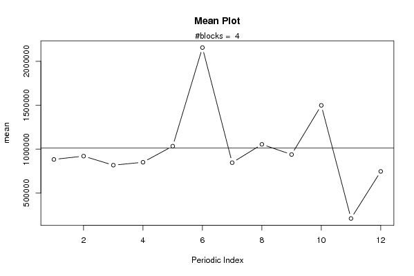
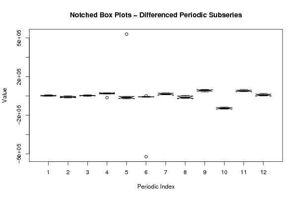
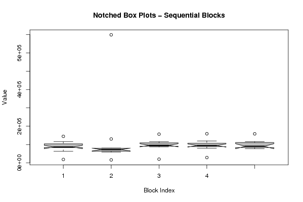
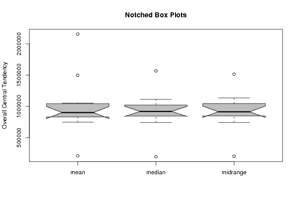
| Title produced by software | Mean Plot | ||||||||||||||||||||
| Date of computation | Tue, 23 Nov 2010 17:09:59 +0000 | ||||||||||||||||||||
| Cite this page as follows | Statistical Computations at FreeStatistics.org, Office for Research Development and Education, URL https://freestatistics.org/blog/index.php?v=date/2010/Nov/23/t129053210197caclpv706psrl.htm/, Retrieved Fri, 26 Apr 2024 22:15:28 +0000 | ||||||||||||||||||||
| Statistical Computations at FreeStatistics.org, Office for Research Development and Education, URL https://freestatistics.org/blog/index.php?pk=99453, Retrieved Fri, 26 Apr 2024 22:15:28 +0000 | |||||||||||||||||||||
| QR Codes: | |||||||||||||||||||||
|
| |||||||||||||||||||||
| Original text written by user: | |||||||||||||||||||||
| IsPrivate? | No (this computation is public) | ||||||||||||||||||||
| User-defined keywords | |||||||||||||||||||||
| Estimated Impact | 148 | ||||||||||||||||||||
Tree of Dependent Computations | |||||||||||||||||||||
| Family? (F = Feedback message, R = changed R code, M = changed R Module, P = changed Parameters, D = changed Data) | |||||||||||||||||||||
| - [Central Tendency] [Arabica Price in ...] [2008-01-19 12:03:37] [74be16979710d4c4e7c6647856088456] - RM D [Mean Plot] [] [2010-11-16 19:28:51] [b98453cac15ba1066b407e146608df68] - PD [Mean Plot] [] [2010-11-23 17:09:59] [27f38de572a508a633f0ad2411de6a3e] [Current] | |||||||||||||||||||||
| Feedback Forum | |||||||||||||||||||||
Post a new message | |||||||||||||||||||||
Dataset | |||||||||||||||||||||
| Dataseries X: | |||||||||||||||||||||
990633 1047696 835567 867169 1161937 846354 852288 1033321 865605 1447252 187910 631074 630867 774318 637859 764244 591077 6990528 693887 807691 802010 1303548 162242 683606 957467 945691 904843 908178 1107174 1049559 960388 1086083 1162190 1568232 201733 871654 963424 930097 940654 883223 1197679 955581 886167 1180383 954937 1589668 291111 800423 873241 906223 768775 833106 1113844 940493 837936 1165387 909788 1584838 | |||||||||||||||||||||
Tables (Output of Computation) | |||||||||||||||||||||
| |||||||||||||||||||||
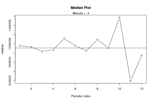
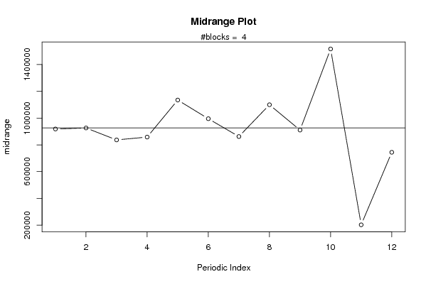
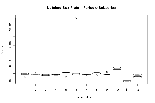
Figures (Output of Computation) | |||||||||||||||||||||
Input Parameters & R Code | |||||||||||||||||||||
| Parameters (Session): | |||||||||||||||||||||
| par1 = 12 ; | |||||||||||||||||||||
| Parameters (R input): | |||||||||||||||||||||
| par1 = 12 ; | |||||||||||||||||||||
| R code (references can be found in the software module): | |||||||||||||||||||||
par1 <- as.numeric(par1) | |||||||||||||||||||||