Repository of Reproducible Computations

Free Statistics

of Irreproducible Research!

Author's title

Author

*The author of this computation has been verified*

R Software Module

rwasp_autocorrelation.wasp

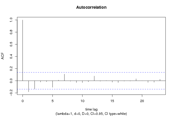
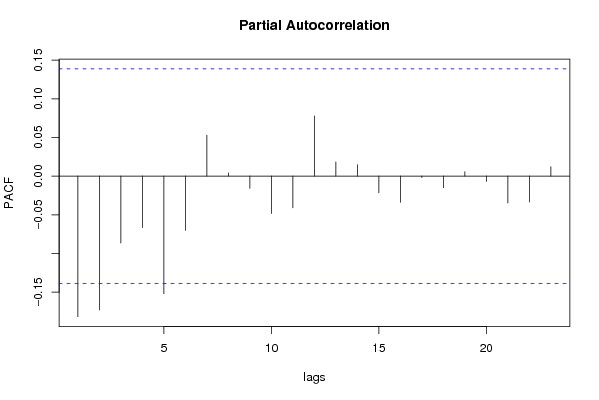
Title produced by software

(Partial) Autocorrelation Function

Date of computation

Tue, 23 Nov 2010 15:32:11 +0000

Cite this page as follows

Statistical Computations at FreeStatistics.org, Office for Research Development and Education, URL https://freestatistics.org/blog/index.php?v=date/2010/Nov/23/t12905263416lat5s9s7osnus5.htm/, Retrieved Tue, 23 Apr 2024 16:45:30 +0000

Statistical Computations at FreeStatistics.org, Office for Research Development and Education, URL https://freestatistics.org/blog/index.php?pk=99282, Retrieved Tue, 23 Apr 2024 16:45:30 +0000

QR Codes:

Paste this QR Code to cite your computation.

Original text written by user:

IsPrivate?

No (this computation is public)

User-defined keywords

Estimated Impact

104

Family? (F = Feedback message, R = changed R code, M = changed R Module, P = changed Parameters, D = changed Data)

-       [(Partial) Autocorrelation Function] [HAR central tendency] [2010-11-23 15:32:11] [f76239c595e4d455b3b05a43389f68d5] [Current]

Feedback Forum

Post a new message

Dataseries X:

Download CSV

Histogram

Boxplots

-0.24320322098871
3.9523939676656E-14
0.24320322098874
-5.7731597280508E-15
-5.7731597280508E-15
-5.7731597280508E-15
-5.7731597280508E-15
-0.24320322098871
3.9523939676656E-14
3.9523939676656E-14
0.01889076246954
-0.018890762469514
3.9523939676656E-14
0.01889076246954
-0.018890762469514
0.01889076246954
-1.4210854715202E-14
-1.4210854715202E-14
-1.4210854715202E-14
-0.077171589615714
-2.0872192862953E-14
-2.0872192862953E-14
-0.010797183330221
4.3076653355456E-14
0.00063836580524335
-0.00063836580522958
4.3076653355456E-14
4.3076653355456E-14
4.3076653355456E-14
4.3076653355456E-14
0.010797183330243
-2.0872192862953E-14
-2.0872192862953E-14
-2.0872192862953E-14
-0.010797183330221
0.010797183330243
-2.0872192862953E-14
-2.0872192862953E-14
-2.0872192862953E-14
-2.0872192862953E-14
-2.0872192862953E-14
-2.0872192862953E-14
-0.010797183330221
0.010797183330243
-2.0872192862953E-14
-2.0872192862953E-14
-2.0872192862953E-14
-2.0872192862953E-14
-2.0872192862953E-14
-2.0872192862953E-14
-2.0872192862953E-14
-2.0872192862953E-14
-2.0872192862953E-14
-2.0872192862953E-14
-2.0872192862953E-14
-2.0872192862953E-14
-2.0872192862953E-14
-0.33710414817462
-0.020563978997795
0.020563978997754
4.8849813083507E-15
4.8849813083507E-15
-0.036039936483195
0.015475957485402
-4.5741188614556E-14
-4.5741188614556E-14
-4.5741188614556E-14
-4.5741188614556E-14
-4.5741188614556E-14
-4.5741188614556E-14
-4.5741188614556E-14
-0.0063434739221457
0.026907452919929
4.8849813083507E-15
-0.020563978997795
-4.5741188614556E-14
-4.5741188614556E-14
-0.021918685707646
8.8817841970013E-16
0.014665707402601
-0.01466570740263
-0.079734968018899
0.094400675421454
-2.9753977059954E-14
-2.9753977059954E-14
-2.9753977059954E-14
-0.01466570740263
8.8817841970013E-16
8.8817841970013E-16
0.014665707402601
-2.9753977059954E-14
-0.01466570740263
-0.0055555698445993
-0.018744691286197
-4.6185277824407E-14
-4.6185277824407E-14
0.018744691286154
2.6645352591004E-15
-0.018744691286197
-0.0056926149932464
-0.01921288685996
3.1086244689504E-14
3.1086244689504E-14
0.00096946202453108
-1.6875389974302E-14
-1.6875389974302E-14
-0.00096946202451687
0.00096946202453108
-1.6875389974302E-14
-0.00096946202451687
3.1086244689504E-14
3.1086244689504E-14
3.1086244689504E-14
3.1086244689504E-14
3.1086244689504E-14
3.1086244689504E-14
3.1086244689504E-14
-0.24125023635047
0.24125023635051
3.1086244689504E-14
3.1086244689504E-14
3.1086244689504E-14
0.019212886860031
4.0412118096356E-14
4.0412118096356E-14
4.0412118096356E-14
-0.01921288685996
3.1086244689504E-14
3.1086244689504E-14
-0.071351199555069
9.3258734068513E-15
9.3258734068513E-15
9.3258734068513E-15
9.3258734068513E-15
-0.01892800988549
2.8421709430404E-14
2.8421709430404E-14
2.8421709430404E-14
2.8421709430404E-14
0.018928009885528
9.3258734068513E-15
-0.01892800988549
-0.034560675065472
-0.011049836186604
-1.9539925233403E-14
-1.9539925233403E-14
-1.9539925233403E-14
0.01104983618658
-4.4408920985006E-15
-4.4408920985006E-15
-4.4408920985006E-15
-4.4408920985006E-15
-4.4408920985006E-15
-0.011049836186604
-0.10043439732182
0.11148423350835
-4.4408920985006E-15
-4.4408920985006E-15
-4.4408920985006E-15
-4.4408920985006E-15
-0.1114842335084
0.11148423350835
-4.4408920985006E-15
-4.4408920985006E-15
-4.4408920985006E-15
-0.1114842335084
-4.8849813083507E-14
-0.017348638334649
0.012422519998564
0.021978906718807
3.1974423109205E-14
3.1974423109205E-14
-0.021978906718768
6.6613381477509E-15
6.6613381477509E-15
6.6613381477509E-15
0.021978906718807
-0.021978906718768
6.6613381477509E-15
6.6613381477509E-15
6.6613381477509E-15
0.021978906718807
3.1974423109205E-14
-0.021978906718768
0.021978906718807
-0.021978906718768
0.021978906718807
3.1974423109205E-14
3.1974423109205E-14
-0.021978906718768
6.6613381477509E-15
0.021978906718807
3.1974423109205E-14
-0.034401426717368
0.034401426717364
3.1974423109205E-14
0.034424764212532
-0.068826190929888
0.068826190929864
1.1546319456102E-14

Summary of computational transaction
Raw Input	view raw input (R code)
Raw Output	view raw output of R engine
Computing time	4 seconds
R Server	'Sir Ronald Aylmer Fisher' @ 193.190.124.24

\begin{tabular}{lllllllll}
\hline
Summary of computational transaction \tabularnewline
Raw Input & view raw input (R code)  \tabularnewline
Raw Output & view raw output of R engine  \tabularnewline
Computing time & 4 seconds \tabularnewline
R Server & 'Sir Ronald Aylmer Fisher' @ 193.190.124.24 \tabularnewline
\hline
\end{tabular}
%Source: https://freestatistics.org/blog/index.php?pk=99282&T=0

[TABLE]
[ROW][C]Summary of computational transaction[/C][/ROW]
[ROW][C]Raw Input[/C][C]view raw input (R code) [/C][/ROW]
[ROW][C]Raw Output[/C][C]view raw output of R engine [/C][/ROW]
[ROW][C]Computing time[/C][C]4 seconds[/C][/ROW]
[ROW][C]R Server[/C][C]'Sir Ronald Aylmer Fisher' @ 193.190.124.24[/C][/ROW]
[/TABLE]
Source: https://freestatistics.org/blog/index.php?pk=99282&T=0

Globally Unique Identifier (entire table): ba.freestatistics.org/blog/index.php?pk=99282&T=0

As an alternative you can also use a QR Code:

The GUIDs for individual cells are displayed in the table below:

Summary of computational transaction
Raw Input	view raw input (R code)
Raw Output	view raw output of R engine
Computing time	4 seconds
R Server	'Sir Ronald Aylmer Fisher' @ 193.190.124.24

Autocorrelation Function
Time lag k	ACF(k)	T-STAT	P-value
1	-0.181753	-2.5704	0.005443
2	-0.134264	-1.8988	0.029516
3	-0.021026	-0.2974	0.383252
4	-0.015624	-0.221	0.412673
5	-0.107493	-1.5202	0.065022
6	0.010478	0.1482	0.441177
7	0.109543	1.5492	0.061461
8	-0.008467	-0.1197	0.452405
9	-0.029809	-0.4216	0.336898
10	-0.03054	-0.4319	0.333138
11	-0.016781	-0.2373	0.406324
12	0.078376	1.1084	0.134508
13	-0.006704	-0.0948	0.462283
14	0.004366	0.0617	0.475412
15	-0.024179	-0.3419	0.366375
16	-0.029416	-0.416	0.338924
17	-0.006121	-0.0866	0.465555
18	-0.00449	-0.0635	0.474715
19	0.033207	0.4696	0.319571
20	0.001521	0.0215	0.49143
21	-0.027885	-0.3943	0.346872
22	-0.025095	-0.3549	0.361519
23	0.025661	0.3629	0.358532

\begin{tabular}{lllllllll}
\hline
Autocorrelation Function \tabularnewline
Time lag k & ACF(k) & T-STAT & P-value \tabularnewline
1 & -0.181753 & -2.5704 & 0.005443 \tabularnewline
2 & -0.134264 & -1.8988 & 0.029516 \tabularnewline
3 & -0.021026 & -0.2974 & 0.383252 \tabularnewline
4 & -0.015624 & -0.221 & 0.412673 \tabularnewline
5 & -0.107493 & -1.5202 & 0.065022 \tabularnewline
6 & 0.010478 & 0.1482 & 0.441177 \tabularnewline
7 & 0.109543 & 1.5492 & 0.061461 \tabularnewline
8 & -0.008467 & -0.1197 & 0.452405 \tabularnewline
9 & -0.029809 & -0.4216 & 0.336898 \tabularnewline
10 & -0.03054 & -0.4319 & 0.333138 \tabularnewline
11 & -0.016781 & -0.2373 & 0.406324 \tabularnewline
12 & 0.078376 & 1.1084 & 0.134508 \tabularnewline
13 & -0.006704 & -0.0948 & 0.462283 \tabularnewline
14 & 0.004366 & 0.0617 & 0.475412 \tabularnewline
15 & -0.024179 & -0.3419 & 0.366375 \tabularnewline
16 & -0.029416 & -0.416 & 0.338924 \tabularnewline
17 & -0.006121 & -0.0866 & 0.465555 \tabularnewline
18 & -0.00449 & -0.0635 & 0.474715 \tabularnewline
19 & 0.033207 & 0.4696 & 0.319571 \tabularnewline
20 & 0.001521 & 0.0215 & 0.49143 \tabularnewline
21 & -0.027885 & -0.3943 & 0.346872 \tabularnewline
22 & -0.025095 & -0.3549 & 0.361519 \tabularnewline
23 & 0.025661 & 0.3629 & 0.358532 \tabularnewline
\hline
\end{tabular}
%Source: https://freestatistics.org/blog/index.php?pk=99282&T=1

[TABLE]
[ROW][C]Autocorrelation Function[/C][/ROW]
[ROW][C]Time lag k[/C][C]ACF(k)[/C][C]T-STAT[/C][C]P-value[/C][/ROW]
[ROW][C]1[/C][C]-0.181753[/C][C]-2.5704[/C][C]0.005443[/C][/ROW]
[ROW][C]2[/C][C]-0.134264[/C][C]-1.8988[/C][C]0.029516[/C][/ROW]
[ROW][C]3[/C][C]-0.021026[/C][C]-0.2974[/C][C]0.383252[/C][/ROW]
[ROW][C]4[/C][C]-0.015624[/C][C]-0.221[/C][C]0.412673[/C][/ROW]
[ROW][C]5[/C][C]-0.107493[/C][C]-1.5202[/C][C]0.065022[/C][/ROW]
[ROW][C]6[/C][C]0.010478[/C][C]0.1482[/C][C]0.441177[/C][/ROW]
[ROW][C]7[/C][C]0.109543[/C][C]1.5492[/C][C]0.061461[/C][/ROW]
[ROW][C]8[/C][C]-0.008467[/C][C]-0.1197[/C][C]0.452405[/C][/ROW]
[ROW][C]9[/C][C]-0.029809[/C][C]-0.4216[/C][C]0.336898[/C][/ROW]
[ROW][C]10[/C][C]-0.03054[/C][C]-0.4319[/C][C]0.333138[/C][/ROW]
[ROW][C]11[/C][C]-0.016781[/C][C]-0.2373[/C][C]0.406324[/C][/ROW]
[ROW][C]12[/C][C]0.078376[/C][C]1.1084[/C][C]0.134508[/C][/ROW]
[ROW][C]13[/C][C]-0.006704[/C][C]-0.0948[/C][C]0.462283[/C][/ROW]
[ROW][C]14[/C][C]0.004366[/C][C]0.0617[/C][C]0.475412[/C][/ROW]
[ROW][C]15[/C][C]-0.024179[/C][C]-0.3419[/C][C]0.366375[/C][/ROW]
[ROW][C]16[/C][C]-0.029416[/C][C]-0.416[/C][C]0.338924[/C][/ROW]
[ROW][C]17[/C][C]-0.006121[/C][C]-0.0866[/C][C]0.465555[/C][/ROW]
[ROW][C]18[/C][C]-0.00449[/C][C]-0.0635[/C][C]0.474715[/C][/ROW]
[ROW][C]19[/C][C]0.033207[/C][C]0.4696[/C][C]0.319571[/C][/ROW]
[ROW][C]20[/C][C]0.001521[/C][C]0.0215[/C][C]0.49143[/C][/ROW]
[ROW][C]21[/C][C]-0.027885[/C][C]-0.3943[/C][C]0.346872[/C][/ROW]
[ROW][C]22[/C][C]-0.025095[/C][C]-0.3549[/C][C]0.361519[/C][/ROW]
[ROW][C]23[/C][C]0.025661[/C][C]0.3629[/C][C]0.358532[/C][/ROW]
[/TABLE]
Source: https://freestatistics.org/blog/index.php?pk=99282&T=1

Globally Unique Identifier (entire table): ba.freestatistics.org/blog/index.php?pk=99282&T=1

As an alternative you can also use a QR Code:

The GUIDs for individual cells are displayed in the table below:

Autocorrelation Function
Time lag k	ACF(k)	T-STAT	P-value
1	-0.181753	-2.5704	0.005443
2	-0.134264	-1.8988	0.029516
3	-0.021026	-0.2974	0.383252
4	-0.015624	-0.221	0.412673
5	-0.107493	-1.5202	0.065022
6	0.010478	0.1482	0.441177
7	0.109543	1.5492	0.061461
8	-0.008467	-0.1197	0.452405
9	-0.029809	-0.4216	0.336898
10	-0.03054	-0.4319	0.333138
11	-0.016781	-0.2373	0.406324
12	0.078376	1.1084	0.134508
13	-0.006704	-0.0948	0.462283
14	0.004366	0.0617	0.475412
15	-0.024179	-0.3419	0.366375
16	-0.029416	-0.416	0.338924
17	-0.006121	-0.0866	0.465555
18	-0.00449	-0.0635	0.474715
19	0.033207	0.4696	0.319571
20	0.001521	0.0215	0.49143
21	-0.027885	-0.3943	0.346872
22	-0.025095	-0.3549	0.361519
23	0.025661	0.3629	0.358532

Partial Autocorrelation Function
Time lag k	PACF(k)	T-STAT	P-value
1	-0.181753	-2.5704	0.005443
2	-0.173014	-2.4468	0.007639
3	-0.086456	-1.2227	0.111447
4	-0.066422	-0.9394	0.174341
5	-0.152288	-2.1537	0.016231
6	-0.069973	-0.9896	0.161791
7	0.052931	0.7486	0.227501
8	0.004143	0.0586	0.47667
9	-0.01566	-0.2215	0.412477
10	-0.048415	-0.6847	0.247164
11	-0.040854	-0.5778	0.282037
12	0.077835	1.1008	0.136163
13	0.018409	0.2603	0.397434
14	0.014754	0.2086	0.417468
15	-0.021615	-0.3057	0.380084
16	-0.033816	-0.4782	0.316502
17	-0.001736	-0.0245	0.49022
18	-0.015073	-0.2132	0.41571
19	0.005728	0.081	0.467761
20	-0.006911	-0.0977	0.461118
21	-0.034699	-0.4907	0.312081
22	-0.033446	-0.473	0.318364
23	0.012096	0.1711	0.432171

\begin{tabular}{lllllllll}
\hline
Partial Autocorrelation Function \tabularnewline
Time lag k & PACF(k) & T-STAT & P-value \tabularnewline
1 & -0.181753 & -2.5704 & 0.005443 \tabularnewline
2 & -0.173014 & -2.4468 & 0.007639 \tabularnewline
3 & -0.086456 & -1.2227 & 0.111447 \tabularnewline
4 & -0.066422 & -0.9394 & 0.174341 \tabularnewline
5 & -0.152288 & -2.1537 & 0.016231 \tabularnewline
6 & -0.069973 & -0.9896 & 0.161791 \tabularnewline
7 & 0.052931 & 0.7486 & 0.227501 \tabularnewline
8 & 0.004143 & 0.0586 & 0.47667 \tabularnewline
9 & -0.01566 & -0.2215 & 0.412477 \tabularnewline
10 & -0.048415 & -0.6847 & 0.247164 \tabularnewline
11 & -0.040854 & -0.5778 & 0.282037 \tabularnewline
12 & 0.077835 & 1.1008 & 0.136163 \tabularnewline
13 & 0.018409 & 0.2603 & 0.397434 \tabularnewline
14 & 0.014754 & 0.2086 & 0.417468 \tabularnewline
15 & -0.021615 & -0.3057 & 0.380084 \tabularnewline
16 & -0.033816 & -0.4782 & 0.316502 \tabularnewline
17 & -0.001736 & -0.0245 & 0.49022 \tabularnewline
18 & -0.015073 & -0.2132 & 0.41571 \tabularnewline
19 & 0.005728 & 0.081 & 0.467761 \tabularnewline
20 & -0.006911 & -0.0977 & 0.461118 \tabularnewline
21 & -0.034699 & -0.4907 & 0.312081 \tabularnewline
22 & -0.033446 & -0.473 & 0.318364 \tabularnewline
23 & 0.012096 & 0.1711 & 0.432171 \tabularnewline
\hline
\end{tabular}
%Source: https://freestatistics.org/blog/index.php?pk=99282&T=2

[TABLE]
[ROW][C]Partial Autocorrelation Function[/C][/ROW]
[ROW][C]Time lag k[/C][C]PACF(k)[/C][C]T-STAT[/C][C]P-value[/C][/ROW]
[ROW][C]1[/C][C]-0.181753[/C][C]-2.5704[/C][C]0.005443[/C][/ROW]
[ROW][C]2[/C][C]-0.173014[/C][C]-2.4468[/C][C]0.007639[/C][/ROW]
[ROW][C]3[/C][C]-0.086456[/C][C]-1.2227[/C][C]0.111447[/C][/ROW]
[ROW][C]4[/C][C]-0.066422[/C][C]-0.9394[/C][C]0.174341[/C][/ROW]
[ROW][C]5[/C][C]-0.152288[/C][C]-2.1537[/C][C]0.016231[/C][/ROW]
[ROW][C]6[/C][C]-0.069973[/C][C]-0.9896[/C][C]0.161791[/C][/ROW]
[ROW][C]7[/C][C]0.052931[/C][C]0.7486[/C][C]0.227501[/C][/ROW]
[ROW][C]8[/C][C]0.004143[/C][C]0.0586[/C][C]0.47667[/C][/ROW]
[ROW][C]9[/C][C]-0.01566[/C][C]-0.2215[/C][C]0.412477[/C][/ROW]
[ROW][C]10[/C][C]-0.048415[/C][C]-0.6847[/C][C]0.247164[/C][/ROW]
[ROW][C]11[/C][C]-0.040854[/C][C]-0.5778[/C][C]0.282037[/C][/ROW]
[ROW][C]12[/C][C]0.077835[/C][C]1.1008[/C][C]0.136163[/C][/ROW]
[ROW][C]13[/C][C]0.018409[/C][C]0.2603[/C][C]0.397434[/C][/ROW]
[ROW][C]14[/C][C]0.014754[/C][C]0.2086[/C][C]0.417468[/C][/ROW]
[ROW][C]15[/C][C]-0.021615[/C][C]-0.3057[/C][C]0.380084[/C][/ROW]
[ROW][C]16[/C][C]-0.033816[/C][C]-0.4782[/C][C]0.316502[/C][/ROW]
[ROW][C]17[/C][C]-0.001736[/C][C]-0.0245[/C][C]0.49022[/C][/ROW]
[ROW][C]18[/C][C]-0.015073[/C][C]-0.2132[/C][C]0.41571[/C][/ROW]
[ROW][C]19[/C][C]0.005728[/C][C]0.081[/C][C]0.467761[/C][/ROW]
[ROW][C]20[/C][C]-0.006911[/C][C]-0.0977[/C][C]0.461118[/C][/ROW]
[ROW][C]21[/C][C]-0.034699[/C][C]-0.4907[/C][C]0.312081[/C][/ROW]
[ROW][C]22[/C][C]-0.033446[/C][C]-0.473[/C][C]0.318364[/C][/ROW]
[ROW][C]23[/C][C]0.012096[/C][C]0.1711[/C][C]0.432171[/C][/ROW]
[/TABLE]
Source: https://freestatistics.org/blog/index.php?pk=99282&T=2

Globally Unique Identifier (entire table): ba.freestatistics.org/blog/index.php?pk=99282&T=2

As an alternative you can also use a QR Code:

The GUIDs for individual cells are displayed in the table below:

Partial Autocorrelation Function
Time lag k	PACF(k)	T-STAT	P-value
1	-0.181753	-2.5704	0.005443
2	-0.173014	-2.4468	0.007639
3	-0.086456	-1.2227	0.111447
4	-0.066422	-0.9394	0.174341
5	-0.152288	-2.1537	0.016231
6	-0.069973	-0.9896	0.161791
7	0.052931	0.7486	0.227501
8	0.004143	0.0586	0.47667
9	-0.01566	-0.2215	0.412477
10	-0.048415	-0.6847	0.247164
11	-0.040854	-0.5778	0.282037
12	0.077835	1.1008	0.136163
13	0.018409	0.2603	0.397434
14	0.014754	0.2086	0.417468
15	-0.021615	-0.3057	0.380084
16	-0.033816	-0.4782	0.316502
17	-0.001736	-0.0245	0.49022
18	-0.015073	-0.2132	0.41571
19	0.005728	0.081	0.467761
20	-0.006911	-0.0977	0.461118
21	-0.034699	-0.4907	0.312081
22	-0.033446	-0.473	0.318364
23	0.012096	0.1711	0.432171

Figure 1

PNG link

Postscript link

PDF link

Figure 2

PNG link

Postscript link

PDF link

Parameters (Session):

par1 = Apollo Oil Corp. ; par3 = Time series of Xycoon Stock Exchange ; par4 = No season ;

Parameters (R input):

par1 = Default ; par2 = 1 ; par3 = 0 ; par4 = 0 ; par5 = 12 ; par6 = White Noise ; par7 = 0.95 ;

R code (references can be found in the software module):

if (par1 == 'Default') {
par1 = 10*log10(length(x))
} else {
par1 <- as.numeric(par1)
}
par2 <- as.numeric(par2)
par3 <- as.numeric(par3)
par4 <- as.numeric(par4)
par5 <- as.numeric(par5)
if (par6 == 'White Noise') par6 <- 'white' else par6 <- 'ma'
par7 <- as.numeric(par7)
if (par2 == 0) {
x <- log(x)
} else {
x <- (x ^ par2 - 1) / par2
}
if (par3 > 0) x <- diff(x,lag=1,difference=par3)
if (par4 > 0) x <- diff(x,lag=par5,difference=par4)
bitmap(file='pic1.png')
racf <- acf(x, par1, main='Autocorrelation', xlab='time lag', ylab='ACF', ci.type=par6, ci=par7, sub=paste('(lambda=',par2,', d=',par3,', D=',par4,', CI=', par7, ', CI type=',par6,')',sep=''))
dev.off()
bitmap(file='pic2.png')
rpacf <- pacf(x,par1,main='Partial Autocorrelation',xlab='lags',ylab='PACF')
dev.off()
(myacf <- c(racf$acf))
(mypacf <- c(rpacf$acf))
lengthx <- length(x)
sqrtn <- sqrt(lengthx)
load(file='createtable')
a<-table.start()
a<-table.row.start(a)
a<-table.element(a,'Autocorrelation Function',4,TRUE)
a<-table.row.end(a)
a<-table.row.start(a)
a<-table.element(a,'Time lag k',header=TRUE)
a<-table.element(a,hyperlink('basics.htm','ACF(k)','click here for more information about the Autocorrelation Function'),header=TRUE)
a<-table.element(a,'T-STAT',header=TRUE)
a<-table.element(a,'P-value',header=TRUE)
a<-table.row.end(a)
for (i in 2:(par1+1)) {
a<-table.row.start(a)
a<-table.element(a,i-1,header=TRUE)
a<-table.element(a,round(myacf[i],6))
mytstat <- myacf[i]*sqrtn
a<-table.element(a,round(mytstat,4))
a<-table.element(a,round(1-pt(abs(mytstat),lengthx),6))
a<-table.row.end(a)
}
a<-table.end(a)
table.save(a,file='mytable.tab')
a<-table.start()
a<-table.row.start(a)
a<-table.element(a,'Partial Autocorrelation Function',4,TRUE)
a<-table.row.end(a)
a<-table.row.start(a)
a<-table.element(a,'Time lag k',header=TRUE)
a<-table.element(a,hyperlink('basics.htm','PACF(k)','click here for more information about the Partial Autocorrelation Function'),header=TRUE)
a<-table.element(a,'T-STAT',header=TRUE)
a<-table.element(a,'P-value',header=TRUE)
a<-table.row.end(a)
for (i in 1:par1) {
a<-table.row.start(a)
a<-table.element(a,i,header=TRUE)
a<-table.element(a,round(mypacf[i],6))
mytstat <- mypacf[i]*sqrtn
a<-table.element(a,round(mytstat,4))
a<-table.element(a,round(1-pt(abs(mytstat),lengthx),6))
a<-table.row.end(a)
}
a<-table.end(a)
table.save(a,file='mytable1.tab')

Free Statistics

Description of Statistical Computation

Tree of Dependent Computations

Dataset

Tables (Output of Computation)

Figures (Output of Computation)

Input Parameters & R Code