Repository of Reproducible Computations

Free Statistics

of Irreproducible Research!

Author's title

Author

*The author of this computation has been verified*

R Software Module

rwasp_autocorrelation.wasp

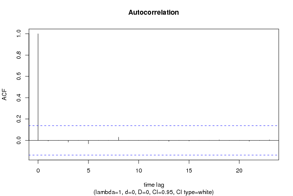
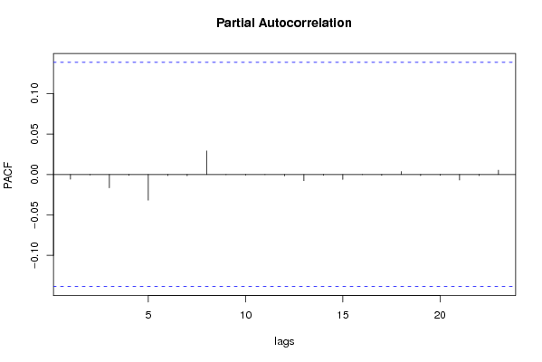
Title produced by software

(Partial) Autocorrelation Function

Date of computation

Tue, 23 Nov 2010 15:17:27 +0000

Cite this page as follows

Statistical Computations at FreeStatistics.org, Office for Research Development and Education, URL https://freestatistics.org/blog/index.php?v=date/2010/Nov/23/t1290525435odkyjmpxl8u49n6.htm/, Retrieved Fri, 19 Apr 2024 07:50:14 +0000

Statistical Computations at FreeStatistics.org, Office for Research Development and Education, URL https://freestatistics.org/blog/index.php?pk=99256, Retrieved Fri, 19 Apr 2024 07:50:14 +0000

QR Codes:

Paste this QR Code to cite your computation.

Original text written by user:

IsPrivate?

No (this computation is public)

User-defined keywords

Estimated Impact

Family? (F = Feedback message, R = changed R code, M = changed R Module, P = changed Parameters, D = changed Data)

-       [(Partial) Autocorrelation Function] [PAP autocorrelation] [2010-11-23 15:17:27] [f76239c595e4d455b3b05a43389f68d5] [Current]

Feedback Forum

Post a new message

Dataseries X:

Download CSV

Histogram

Boxplots

-3.3306690738755E-14
0.0053840193399668
3.3750779948605E-14
3.3750779948605E-14
-0.0053840193399664
-3.3306690738755E-14
-3.3306690738755E-14
0.0053840193399668
-0.021066849967766
-4.6185277824407E-14
0.021066849967754
3.3750779948605E-14
3.3750779948605E-14
3.3750779948605E-14
3.3750779948605E-14
3.3750779948605E-14
3.3750779948605E-14
3.3750779948605E-14
3.3750779948605E-14
3.3750779948605E-14
3.3750779948605E-14
3.3750779948605E-14
3.3750779948605E-14
3.3750779948605E-14
3.3750779948605E-14
-0.0053840193399664
0.0053840193399668
3.3750779948605E-14
3.3750779948605E-14
3.3750779948605E-14
3.3750779948605E-14
3.3750779948605E-14
-0.0053840193399664
-3.3306690738755E-14
-3.3306690738755E-14
-3.3306690738755E-14
0.0053840193399668
3.3750779948605E-14
-0.0053840193399664
-3.3306690738755E-14
-3.3306690738755E-14
-3.3306690738755E-14
-3.3306690738755E-14
-3.3306690738755E-14
-3.3306690738755E-14
0.0053840193399668
3.3750779948605E-14
3.3750779948605E-14
-0.0053840193399664
0.0053840193399668
3.3750779948605E-14
3.3750779948605E-14
-0.0053840193399664
-3.3306690738755E-14
-3.3306690738755E-14
-3.3306690738755E-14
-3.3306690738755E-14
0.0053840193399668
3.3750779948605E-14
3.3750779948605E-14
3.3750779948605E-14
-0.0053840193399664
-3.3306690738755E-14
-3.3306690738755E-14
-3.3306690738755E-14
0.0053840193399668
3.3750779948605E-14
3.3750779948605E-14
3.3750779948605E-14
3.3750779948605E-14
3.3750779948605E-14
3.3750779948605E-14
3.3750779948605E-14
3.3750779948605E-14
3.3750779948605E-14
0.0003158060976336
-4.8405723873657E-14
-4.8405723873657E-14
-4.8405723873657E-14
-4.8405723873657E-14
-0.0056998254376484
-3.3306690738755E-14
0.0056998254375666
-0.0056998254376484
-3.3306690738755E-14
-3.3306690738755E-14
0.0056998254375666
-4.8405723873657E-14
-4.8405723873657E-14
-0.010155593471648
-0.0051167364592297
-1.1990408665952E-14
-1.1990408665952E-14
-1.1990408665952E-14
0.005116736459188
-2.9753977059954E-14
-2.9753977059954E-14
-2.9753977059954E-14
-2.9753977059954E-14
-2.9753977059954E-14
-2.9753977059954E-14
-2.9753977059954E-14
-0.0051167364592297
-1.1990408665952E-14
-1.1990408665952E-14
0.005116736459188
-2.9753977059954E-14
-0.0051167364592297
-1.1990408665952E-14
-1.1990408665952E-14
0.005116736459188
-2.9753977059954E-14
-0.0051167364592297
-1.1990408665952E-14
0.005116736459188
-2.9753977059954E-14
-0.0051167364592297
-0.070734872477612
-3.6859404417555E-14
-3.6859404417555E-14
-3.6859404417555E-14
0.0061749767394632
-0.0061749767394774
-3.6859404417555E-14
-3.6859404417555E-14
-3.6859404417555E-14
-3.6859404417555E-14
-3.6859404417555E-14
-3.6859404417555E-14
0.0061749767394632
-0.0061749767394774
-3.6859404417555E-14
-3.6859404417555E-14
-0.038587740776537
-9.7699626167014E-15
-9.7699626167014E-15
-9.7699626167014E-15
-0.0068186160469095
0.0068186160468917
-9.7699626167014E-15
-0.0068186160469095
-7.9936057773011E-15
-7.9936057773011E-15
-7.9936057773011E-15
0.0068186160468917
-9.7699626167014E-15
-0.0068186160469095
-7.9936057773011E-15
-0.028119435314408
-2.9309887850104E-14
-2.9309887850104E-14
0.028119435314371
-7.9936057773011E-15
-7.9936057773011E-15
-7.9936057773011E-15
-7.9936057773011E-15
0.0068186160468917
-9.7699626167014E-15
-0.0068186160469095
-7.9936057773011E-15
-7.9936057773011E-15
0.0068186160468917
-0.0068186160469095
-7.9936057773011E-15
-7.9936057773011E-15
0.0068186160468917
-0.0068186160469095
-7.9936057773011E-15
-7.9936057773011E-15
-7.9936057773011E-15
-7.9936057773011E-15
-7.9936057773011E-15
-7.9936057773011E-15
-7.9936057773011E-15
0.0068186160468917
-0.0068186160469095
-7.9936057773011E-15
0.0068186160468917
-9.7699626167014E-15
-9.7699626167014E-15
-0.0068186160469095
-7.9936057773011E-15
-7.9936057773011E-15
0.0068186160468917
-9.7699626167014E-15
0.0099644952593905
-4.1300296516056E-14
-4.1300296516056E-14
-4.1300296516056E-14
-4.1300296516056E-14
-0.034585579649741
3.8635761256955E-14
3.8635761256955E-14
0.034585579649739
-4.1300296516056E-14
0.015809217368258
2.6201263381154E-14
2.6201263381154E-14
-1.1179688669752
-3.3306690738755E-14

Summary of computational transaction
Raw Input	view raw input (R code)
Raw Output	view raw output of R engine
Computing time	8 seconds
R Server	'George Udny Yule' @ 72.249.76.132

\begin{tabular}{lllllllll}
\hline
Summary of computational transaction \tabularnewline
Raw Input & view raw input (R code)  \tabularnewline
Raw Output & view raw output of R engine  \tabularnewline
Computing time & 8 seconds \tabularnewline
R Server & 'George Udny Yule' @ 72.249.76.132 \tabularnewline
\hline
\end{tabular}
%Source: https://freestatistics.org/blog/index.php?pk=99256&T=0

[TABLE]
[ROW][C]Summary of computational transaction[/C][/ROW]
[ROW][C]Raw Input[/C][C]view raw input (R code) [/C][/ROW]
[ROW][C]Raw Output[/C][C]view raw output of R engine [/C][/ROW]
[ROW][C]Computing time[/C][C]8 seconds[/C][/ROW]
[ROW][C]R Server[/C][C]'George Udny Yule' @ 72.249.76.132[/C][/ROW]
[/TABLE]
Source: https://freestatistics.org/blog/index.php?pk=99256&T=0

Globally Unique Identifier (entire table): ba.freestatistics.org/blog/index.php?pk=99256&T=0

As an alternative you can also use a QR Code:

The GUIDs for individual cells are displayed in the table below:

Summary of computational transaction
Raw Input	view raw input (R code)
Raw Output	view raw output of R engine
Computing time	8 seconds
R Server	'George Udny Yule' @ 72.249.76.132

Autocorrelation Function
Time lag k	ACF(k)	T-STAT	P-value
1	-0.00591	-0.0836	0.466739
2	-0.000525	-0.0074	0.497042
3	-0.016478	-0.233	0.407986
4	-0.000908	-0.0128	0.494886
5	-0.031784	-0.4495	0.326781
6	-0.000706	-0.01	0.496022
7	-0.001385	-0.0196	0.492197
8	0.030059	0.4251	0.335612
9	-0.000515	-0.0073	0.497099
10	0.000185	0.0026	0.498956
11	-0.001104	-0.0156	0.49378
12	-0.001615	-0.0228	0.490899
13	-0.009526	-0.1347	0.446487
14	-0.000861	-0.0122	0.495149
15	-0.006135	-0.0868	0.465471
16	0.00112	0.0158	0.49369
17	-0.001048	-0.0148	0.494097
18	0.004328	0.0612	0.47563
19	-0.001472	-0.0208	0.491707
20	-0.000831	-0.0118	0.495318
21	-0.007514	-0.1063	0.457738
22	-0.001228	-0.0174	0.493083
23	0.004769	0.0674	0.473146

\begin{tabular}{lllllllll}
\hline
Autocorrelation Function \tabularnewline
Time lag k & ACF(k) & T-STAT & P-value \tabularnewline
1 & -0.00591 & -0.0836 & 0.466739 \tabularnewline
2 & -0.000525 & -0.0074 & 0.497042 \tabularnewline
3 & -0.016478 & -0.233 & 0.407986 \tabularnewline
4 & -0.000908 & -0.0128 & 0.494886 \tabularnewline
5 & -0.031784 & -0.4495 & 0.326781 \tabularnewline
6 & -0.000706 & -0.01 & 0.496022 \tabularnewline
7 & -0.001385 & -0.0196 & 0.492197 \tabularnewline
8 & 0.030059 & 0.4251 & 0.335612 \tabularnewline
9 & -0.000515 & -0.0073 & 0.497099 \tabularnewline
10 & 0.000185 & 0.0026 & 0.498956 \tabularnewline
11 & -0.001104 & -0.0156 & 0.49378 \tabularnewline
12 & -0.001615 & -0.0228 & 0.490899 \tabularnewline
13 & -0.009526 & -0.1347 & 0.446487 \tabularnewline
14 & -0.000861 & -0.0122 & 0.495149 \tabularnewline
15 & -0.006135 & -0.0868 & 0.465471 \tabularnewline
16 & 0.00112 & 0.0158 & 0.49369 \tabularnewline
17 & -0.001048 & -0.0148 & 0.494097 \tabularnewline
18 & 0.004328 & 0.0612 & 0.47563 \tabularnewline
19 & -0.001472 & -0.0208 & 0.491707 \tabularnewline
20 & -0.000831 & -0.0118 & 0.495318 \tabularnewline
21 & -0.007514 & -0.1063 & 0.457738 \tabularnewline
22 & -0.001228 & -0.0174 & 0.493083 \tabularnewline
23 & 0.004769 & 0.0674 & 0.473146 \tabularnewline
\hline
\end{tabular}
%Source: https://freestatistics.org/blog/index.php?pk=99256&T=1

[TABLE]
[ROW][C]Autocorrelation Function[/C][/ROW]
[ROW][C]Time lag k[/C][C]ACF(k)[/C][C]T-STAT[/C][C]P-value[/C][/ROW]
[ROW][C]1[/C][C]-0.00591[/C][C]-0.0836[/C][C]0.466739[/C][/ROW]
[ROW][C]2[/C][C]-0.000525[/C][C]-0.0074[/C][C]0.497042[/C][/ROW]
[ROW][C]3[/C][C]-0.016478[/C][C]-0.233[/C][C]0.407986[/C][/ROW]
[ROW][C]4[/C][C]-0.000908[/C][C]-0.0128[/C][C]0.494886[/C][/ROW]
[ROW][C]5[/C][C]-0.031784[/C][C]-0.4495[/C][C]0.326781[/C][/ROW]
[ROW][C]6[/C][C]-0.000706[/C][C]-0.01[/C][C]0.496022[/C][/ROW]
[ROW][C]7[/C][C]-0.001385[/C][C]-0.0196[/C][C]0.492197[/C][/ROW]
[ROW][C]8[/C][C]0.030059[/C][C]0.4251[/C][C]0.335612[/C][/ROW]
[ROW][C]9[/C][C]-0.000515[/C][C]-0.0073[/C][C]0.497099[/C][/ROW]
[ROW][C]10[/C][C]0.000185[/C][C]0.0026[/C][C]0.498956[/C][/ROW]
[ROW][C]11[/C][C]-0.001104[/C][C]-0.0156[/C][C]0.49378[/C][/ROW]
[ROW][C]12[/C][C]-0.001615[/C][C]-0.0228[/C][C]0.490899[/C][/ROW]
[ROW][C]13[/C][C]-0.009526[/C][C]-0.1347[/C][C]0.446487[/C][/ROW]
[ROW][C]14[/C][C]-0.000861[/C][C]-0.0122[/C][C]0.495149[/C][/ROW]
[ROW][C]15[/C][C]-0.006135[/C][C]-0.0868[/C][C]0.465471[/C][/ROW]
[ROW][C]16[/C][C]0.00112[/C][C]0.0158[/C][C]0.49369[/C][/ROW]
[ROW][C]17[/C][C]-0.001048[/C][C]-0.0148[/C][C]0.494097[/C][/ROW]
[ROW][C]18[/C][C]0.004328[/C][C]0.0612[/C][C]0.47563[/C][/ROW]
[ROW][C]19[/C][C]-0.001472[/C][C]-0.0208[/C][C]0.491707[/C][/ROW]
[ROW][C]20[/C][C]-0.000831[/C][C]-0.0118[/C][C]0.495318[/C][/ROW]
[ROW][C]21[/C][C]-0.007514[/C][C]-0.1063[/C][C]0.457738[/C][/ROW]
[ROW][C]22[/C][C]-0.001228[/C][C]-0.0174[/C][C]0.493083[/C][/ROW]
[ROW][C]23[/C][C]0.004769[/C][C]0.0674[/C][C]0.473146[/C][/ROW]
[/TABLE]
Source: https://freestatistics.org/blog/index.php?pk=99256&T=1

Globally Unique Identifier (entire table): ba.freestatistics.org/blog/index.php?pk=99256&T=1

As an alternative you can also use a QR Code:

The GUIDs for individual cells are displayed in the table below:

Autocorrelation Function
Time lag k	ACF(k)	T-STAT	P-value
1	-0.00591	-0.0836	0.466739
2	-0.000525	-0.0074	0.497042
3	-0.016478	-0.233	0.407986
4	-0.000908	-0.0128	0.494886
5	-0.031784	-0.4495	0.326781
6	-0.000706	-0.01	0.496022
7	-0.001385	-0.0196	0.492197
8	0.030059	0.4251	0.335612
9	-0.000515	-0.0073	0.497099
10	0.000185	0.0026	0.498956
11	-0.001104	-0.0156	0.49378
12	-0.001615	-0.0228	0.490899
13	-0.009526	-0.1347	0.446487
14	-0.000861	-0.0122	0.495149
15	-0.006135	-0.0868	0.465471
16	0.00112	0.0158	0.49369
17	-0.001048	-0.0148	0.494097
18	0.004328	0.0612	0.47563
19	-0.001472	-0.0208	0.491707
20	-0.000831	-0.0118	0.495318
21	-0.007514	-0.1063	0.457738
22	-0.001228	-0.0174	0.493083
23	0.004769	0.0674	0.473146

Partial Autocorrelation Function
Time lag k	PACF(k)	T-STAT	P-value
1	-0.00591	-0.0836	0.466739
2	-0.00056	-0.0079	0.496845
3	-0.016485	-0.2331	0.407947
4	-0.001103	-0.0156	0.493784
5	-0.031825	-0.4501	0.326571
6	-0.00136	-0.0192	0.492339
7	-0.00149	-0.0211	0.491605
8	0.029027	0.4105	0.340938
9	-0.000269	-0.0038	0.498486
10	-0.000812	-0.0115	0.495425
11	-0.000229	-0.0032	0.49871
12	-0.001661	-0.0235	0.490641
13	-0.007712	-0.1091	0.456631
14	-0.000957	-0.0135	0.494607
15	-0.006173	-0.0873	0.465258
16	-0.000144	-0.002	0.499186
17	-0.001189	-0.0168	0.493298
18	0.003605	0.051	0.479696
19	-0.00147	-0.0208	0.491717
20	-0.001186	-0.0168	0.493315
21	-0.006906	-0.0977	0.46115
22	-0.001395	-0.0197	0.492141
23	0.005309	0.0751	0.470114

\begin{tabular}{lllllllll}
\hline
Partial Autocorrelation Function \tabularnewline
Time lag k & PACF(k) & T-STAT & P-value \tabularnewline
1 & -0.00591 & -0.0836 & 0.466739 \tabularnewline
2 & -0.00056 & -0.0079 & 0.496845 \tabularnewline
3 & -0.016485 & -0.2331 & 0.407947 \tabularnewline
4 & -0.001103 & -0.0156 & 0.493784 \tabularnewline
5 & -0.031825 & -0.4501 & 0.326571 \tabularnewline
6 & -0.00136 & -0.0192 & 0.492339 \tabularnewline
7 & -0.00149 & -0.0211 & 0.491605 \tabularnewline
8 & 0.029027 & 0.4105 & 0.340938 \tabularnewline
9 & -0.000269 & -0.0038 & 0.498486 \tabularnewline
10 & -0.000812 & -0.0115 & 0.495425 \tabularnewline
11 & -0.000229 & -0.0032 & 0.49871 \tabularnewline
12 & -0.001661 & -0.0235 & 0.490641 \tabularnewline
13 & -0.007712 & -0.1091 & 0.456631 \tabularnewline
14 & -0.000957 & -0.0135 & 0.494607 \tabularnewline
15 & -0.006173 & -0.0873 & 0.465258 \tabularnewline
16 & -0.000144 & -0.002 & 0.499186 \tabularnewline
17 & -0.001189 & -0.0168 & 0.493298 \tabularnewline
18 & 0.003605 & 0.051 & 0.479696 \tabularnewline
19 & -0.00147 & -0.0208 & 0.491717 \tabularnewline
20 & -0.001186 & -0.0168 & 0.493315 \tabularnewline
21 & -0.006906 & -0.0977 & 0.46115 \tabularnewline
22 & -0.001395 & -0.0197 & 0.492141 \tabularnewline
23 & 0.005309 & 0.0751 & 0.470114 \tabularnewline
\hline
\end{tabular}
%Source: https://freestatistics.org/blog/index.php?pk=99256&T=2

[TABLE]
[ROW][C]Partial Autocorrelation Function[/C][/ROW]
[ROW][C]Time lag k[/C][C]PACF(k)[/C][C]T-STAT[/C][C]P-value[/C][/ROW]
[ROW][C]1[/C][C]-0.00591[/C][C]-0.0836[/C][C]0.466739[/C][/ROW]
[ROW][C]2[/C][C]-0.00056[/C][C]-0.0079[/C][C]0.496845[/C][/ROW]
[ROW][C]3[/C][C]-0.016485[/C][C]-0.2331[/C][C]0.407947[/C][/ROW]
[ROW][C]4[/C][C]-0.001103[/C][C]-0.0156[/C][C]0.493784[/C][/ROW]
[ROW][C]5[/C][C]-0.031825[/C][C]-0.4501[/C][C]0.326571[/C][/ROW]
[ROW][C]6[/C][C]-0.00136[/C][C]-0.0192[/C][C]0.492339[/C][/ROW]
[ROW][C]7[/C][C]-0.00149[/C][C]-0.0211[/C][C]0.491605[/C][/ROW]
[ROW][C]8[/C][C]0.029027[/C][C]0.4105[/C][C]0.340938[/C][/ROW]
[ROW][C]9[/C][C]-0.000269[/C][C]-0.0038[/C][C]0.498486[/C][/ROW]
[ROW][C]10[/C][C]-0.000812[/C][C]-0.0115[/C][C]0.495425[/C][/ROW]
[ROW][C]11[/C][C]-0.000229[/C][C]-0.0032[/C][C]0.49871[/C][/ROW]
[ROW][C]12[/C][C]-0.001661[/C][C]-0.0235[/C][C]0.490641[/C][/ROW]
[ROW][C]13[/C][C]-0.007712[/C][C]-0.1091[/C][C]0.456631[/C][/ROW]
[ROW][C]14[/C][C]-0.000957[/C][C]-0.0135[/C][C]0.494607[/C][/ROW]
[ROW][C]15[/C][C]-0.006173[/C][C]-0.0873[/C][C]0.465258[/C][/ROW]
[ROW][C]16[/C][C]-0.000144[/C][C]-0.002[/C][C]0.499186[/C][/ROW]
[ROW][C]17[/C][C]-0.001189[/C][C]-0.0168[/C][C]0.493298[/C][/ROW]
[ROW][C]18[/C][C]0.003605[/C][C]0.051[/C][C]0.479696[/C][/ROW]
[ROW][C]19[/C][C]-0.00147[/C][C]-0.0208[/C][C]0.491717[/C][/ROW]
[ROW][C]20[/C][C]-0.001186[/C][C]-0.0168[/C][C]0.493315[/C][/ROW]
[ROW][C]21[/C][C]-0.006906[/C][C]-0.0977[/C][C]0.46115[/C][/ROW]
[ROW][C]22[/C][C]-0.001395[/C][C]-0.0197[/C][C]0.492141[/C][/ROW]
[ROW][C]23[/C][C]0.005309[/C][C]0.0751[/C][C]0.470114[/C][/ROW]
[/TABLE]
Source: https://freestatistics.org/blog/index.php?pk=99256&T=2

Globally Unique Identifier (entire table): ba.freestatistics.org/blog/index.php?pk=99256&T=2

As an alternative you can also use a QR Code:

The GUIDs for individual cells are displayed in the table below:

Partial Autocorrelation Function
Time lag k	PACF(k)	T-STAT	P-value
1	-0.00591	-0.0836	0.466739
2	-0.00056	-0.0079	0.496845
3	-0.016485	-0.2331	0.407947
4	-0.001103	-0.0156	0.493784
5	-0.031825	-0.4501	0.326571
6	-0.00136	-0.0192	0.492339
7	-0.00149	-0.0211	0.491605
8	0.029027	0.4105	0.340938
9	-0.000269	-0.0038	0.498486
10	-0.000812	-0.0115	0.495425
11	-0.000229	-0.0032	0.49871
12	-0.001661	-0.0235	0.490641
13	-0.007712	-0.1091	0.456631
14	-0.000957	-0.0135	0.494607
15	-0.006173	-0.0873	0.465258
16	-0.000144	-0.002	0.499186
17	-0.001189	-0.0168	0.493298
18	0.003605	0.051	0.479696
19	-0.00147	-0.0208	0.491717
20	-0.001186	-0.0168	0.493315
21	-0.006906	-0.0977	0.46115
22	-0.001395	-0.0197	0.492141
23	0.005309	0.0751	0.470114

Figure 1

PNG link

Postscript link

PDF link

Figure 2

PNG link

Postscript link

PDF link

Parameters (Session):

par1 = Default ; par2 = 1 ; par3 = 0 ; par4 = 0 ; par5 = 12 ; par6 = White Noise ; par7 = 0.95 ;

Parameters (R input):

par1 = Default ; par2 = 1 ; par3 = 0 ; par4 = 0 ; par5 = 12 ; par6 = White Noise ; par7 = 0.95 ;

R code (references can be found in the software module):

if (par1 == 'Default') {
par1 = 10*log10(length(x))
} else {
par1 <- as.numeric(par1)
}
par2 <- as.numeric(par2)
par3 <- as.numeric(par3)
par4 <- as.numeric(par4)
par5 <- as.numeric(par5)
if (par6 == 'White Noise') par6 <- 'white' else par6 <- 'ma'
par7 <- as.numeric(par7)
if (par2 == 0) {
x <- log(x)
} else {
x <- (x ^ par2 - 1) / par2
}
if (par3 > 0) x <- diff(x,lag=1,difference=par3)
if (par4 > 0) x <- diff(x,lag=par5,difference=par4)
bitmap(file='pic1.png')
racf <- acf(x, par1, main='Autocorrelation', xlab='time lag', ylab='ACF', ci.type=par6, ci=par7, sub=paste('(lambda=',par2,', d=',par3,', D=',par4,', CI=', par7, ', CI type=',par6,')',sep=''))
dev.off()
bitmap(file='pic2.png')
rpacf <- pacf(x,par1,main='Partial Autocorrelation',xlab='lags',ylab='PACF')
dev.off()
(myacf <- c(racf$acf))
(mypacf <- c(rpacf$acf))
lengthx <- length(x)
sqrtn <- sqrt(lengthx)
load(file='createtable')
a<-table.start()
a<-table.row.start(a)
a<-table.element(a,'Autocorrelation Function',4,TRUE)
a<-table.row.end(a)
a<-table.row.start(a)
a<-table.element(a,'Time lag k',header=TRUE)
a<-table.element(a,hyperlink('basics.htm','ACF(k)','click here for more information about the Autocorrelation Function'),header=TRUE)
a<-table.element(a,'T-STAT',header=TRUE)
a<-table.element(a,'P-value',header=TRUE)
a<-table.row.end(a)
for (i in 2:(par1+1)) {
a<-table.row.start(a)
a<-table.element(a,i-1,header=TRUE)
a<-table.element(a,round(myacf[i],6))
mytstat <- myacf[i]*sqrtn
a<-table.element(a,round(mytstat,4))
a<-table.element(a,round(1-pt(abs(mytstat),lengthx),6))
a<-table.row.end(a)
}
a<-table.end(a)
table.save(a,file='mytable.tab')
a<-table.start()
a<-table.row.start(a)
a<-table.element(a,'Partial Autocorrelation Function',4,TRUE)
a<-table.row.end(a)
a<-table.row.start(a)
a<-table.element(a,'Time lag k',header=TRUE)
a<-table.element(a,hyperlink('basics.htm','PACF(k)','click here for more information about the Partial Autocorrelation Function'),header=TRUE)
a<-table.element(a,'T-STAT',header=TRUE)
a<-table.element(a,'P-value',header=TRUE)
a<-table.row.end(a)
for (i in 1:par1) {
a<-table.row.start(a)
a<-table.element(a,i,header=TRUE)
a<-table.element(a,round(mypacf[i],6))
mytstat <- mypacf[i]*sqrtn
a<-table.element(a,round(mytstat,4))
a<-table.element(a,round(1-pt(abs(mytstat),lengthx),6))
a<-table.row.end(a)
}
a<-table.end(a)
table.save(a,file='mytable1.tab')

Free Statistics

Description of Statistical Computation

Tree of Dependent Computations

Dataset

Tables (Output of Computation)

Figures (Output of Computation)

Input Parameters & R Code