Repository of Reproducible Computations

Free Statistics

of Irreproducible Research!

Author's title

Author

*The author of this computation has been verified*

R Software Module

rwasp_autocorrelation.wasp

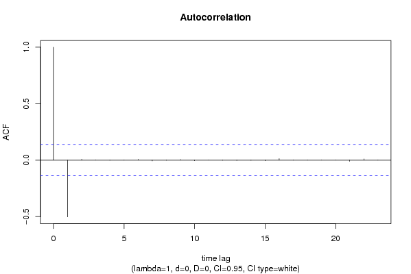
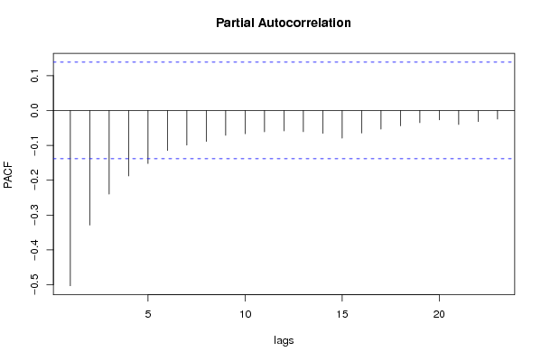
Title produced by software

(Partial) Autocorrelation Function

Date of computation

Tue, 23 Nov 2010 15:07:14 +0000

Cite this page as follows

Statistical Computations at FreeStatistics.org, Office for Research Development and Education, URL https://freestatistics.org/blog/index.php?v=date/2010/Nov/23/t1290524810j0ncx96mfa882f3.htm/, Retrieved Thu, 25 Apr 2024 13:00:11 +0000

Statistical Computations at FreeStatistics.org, Office for Research Development and Education, URL https://freestatistics.org/blog/index.php?pk=99231, Retrieved Thu, 25 Apr 2024 13:00:11 +0000

QR Codes:

Paste this QR Code to cite your computation.

Original text written by user:

IsPrivate?

No (this computation is public)

User-defined keywords

Estimated Impact

110

Family? (F = Feedback message, R = changed R code, M = changed R Module, P = changed Parameters, D = changed Data)

-       [(Partial) Autocorrelation Function] [GRB autocorrelation] [2010-11-23 15:07:14] [f76239c595e4d455b3b05a43389f68d5] [Current]

Feedback Forum

Post a new message

Dataseries X:

Download CSV

Histogram

Boxplots

4.2632564145606E-14
0.0051001932048425
2.2204460492503E-15
2.2204460492503E-15
2.2204460492503E-15
2.2204460492503E-15
2.2204460492503E-15
2.2204460492503E-15
-0.010226531783798
3.3750779948605E-14
3.3750779948605E-14
3.3750779948605E-14
3.3750779948605E-14
0.010226531783834
-0.6758556834499
0.66342407910779
4.7517545453957E-14
4.7517545453957E-14
4.7517545453957E-14
4.7517545453957E-14
4.7517545453957E-14
4.7517545453957E-14
4.7517545453957E-14
4.7517545453957E-14
0.0080616046710476
2.0872192862953E-14
2.0872192862953E-14
2.0872192862953E-14
2.0872192862953E-14
-0.0080616046709792
-0.018567187675552
2.2204460492503E-14
2.2204460492503E-14
2.2204460492503E-14
2.2204460492503E-14
2.2204460492503E-14
-0.013585114590278
2.8865798640254E-14
2.8865798640254E-14
0.013585114590329
2.2204460492503E-14
2.2204460492503E-14
2.2204460492503E-14
2.2204460492503E-14
2.2204460492503E-14
-0.013585114590278
0.013585114590329
-0.0075244899785778
3.7747582837255E-14
3.7747582837255E-14
3.7747582837255E-14
3.7747582837255E-14
3.7747582837255E-14
-0.014454416740162
-2.2204460492503E-15
-0.024041483624702
-0.014229489103917
0.014229489103947
-0.039220713153317
-3.5971225997855E-14
-3.5971225997855E-14
-3.5971225997855E-14
0.015391150320264
-3.3306690738755E-14
-3.3306690738755E-14
-3.3306690738755E-14
-3.3306690738755E-14
-3.3306690738755E-14
-3.3306690738755E-14
-3.3306690738755E-14
-3.3306690738755E-14
-3.3306690738755E-14
-0.015391150320333
-0.0098442140347359
4.1300296516056E-14
-0.013278203386059
1.8207657603853E-14
1.8207657603853E-14
0.013278203386118
4.1300296516056E-14
4.1300296516056E-14
4.1300296516056E-14
4.1300296516056E-14
-0.013278203386059
1.8207657603853E-14
1.8207657603853E-14
1.8207657603853E-14
1.8207657603853E-14
1.8207657603853E-14
1.8207657603853E-14
0.013278203386118
-0.013278203386059
0.013278203386118
4.1300296516056E-14
4.1300296516056E-14
4.1300296516056E-14
4.1300296516056E-14
4.1300296516056E-14
-0.013278203386059
1.8207657603853E-14
1.8207657603853E-14
1.8207657603853E-14
1.8207657603853E-14
0.013278203386118
4.1300296516056E-14
4.1300296516056E-14
-0.013278203386059
1.8207657603853E-14
1.8207657603853E-14
1.8207657603853E-14
0.013278203386118
-0.013278203386059
1.8207657603853E-14
1.8207657603853E-14
0.013278203386118
4.1300296516056E-14
-0.025043044965659
0.0058997221272046
1.6431300764452E-14
1.6431300764452E-14
1.6431300764452E-14
1.6431300764452E-14
1.6431300764452E-14
0.010865129869116
1.2434497875802E-14
1.2434497875802E-14
1.2434497875802E-14
1.2434497875802E-14
1.2434497875802E-14
1.2434497875802E-14
1.2434497875802E-14
-0.026106745837688
-0.015477523068867
0.015477523068947
3.3306690738755E-14
-0.015477523068867
0.015477523068947
-0.015477523068867
4.6629367034257E-14
4.6629367034257E-14
0.015477523068947
3.3306690738755E-14
3.3306690738755E-14
3.3306690738755E-14
-0.015477523068867
4.6629367034257E-14
4.6629367034257E-14
4.6629367034257E-14
4.6629367034257E-14
4.6629367034257E-14
4.6629367034257E-14
4.6629367034257E-14
4.6629367034257E-14
4.6629367034257E-14
4.6629367034257E-14
4.6629367034257E-14
4.6629367034257E-14
4.6629367034257E-14
4.6629367034257E-14
4.6629367034257E-14
0.015477523068947
3.3306690738755E-14
3.3306690738755E-14
3.3306690738755E-14
-0.015477523068867
4.6629367034257E-14
4.6629367034257E-14
4.6629367034257E-14
4.6629367034257E-14
4.6629367034257E-14
0.015477523068947
-0.015477523068867
4.6629367034257E-14
4.6629367034257E-14
4.6629367034257E-14
4.6629367034257E-14
4.6629367034257E-14
4.6629367034257E-14
4.6629367034257E-14
4.6629367034257E-14
4.6629367034257E-14
4.6629367034257E-14
4.6629367034257E-14
4.6629367034257E-14
4.6629367034257E-14
4.6629367034257E-14
4.6629367034257E-14
4.6629367034257E-14
4.6629367034257E-14
0.015477523068947
3.3306690738755E-14
-0.015477523068867
4.6629367034257E-14
4.6629367034257E-14
4.6629367034257E-14
4.6629367034257E-14
4.6629367034257E-14
4.6629367034257E-14
4.6629367034257E-14
0.015477523068947

Summary of computational transaction
Raw Input	view raw input (R code)
Raw Output	view raw output of R engine
Computing time	2 seconds
R Server	'Gwilym Jenkins' @ 72.249.127.135

\begin{tabular}{lllllllll}
\hline
Summary of computational transaction \tabularnewline
Raw Input & view raw input (R code)  \tabularnewline
Raw Output & view raw output of R engine  \tabularnewline
Computing time & 2 seconds \tabularnewline
R Server & 'Gwilym Jenkins' @ 72.249.127.135 \tabularnewline
\hline
\end{tabular}
%Source: https://freestatistics.org/blog/index.php?pk=99231&T=0

[TABLE]
[ROW][C]Summary of computational transaction[/C][/ROW]
[ROW][C]Raw Input[/C][C]view raw input (R code) [/C][/ROW]
[ROW][C]Raw Output[/C][C]view raw output of R engine [/C][/ROW]
[ROW][C]Computing time[/C][C]2 seconds[/C][/ROW]
[ROW][C]R Server[/C][C]'Gwilym Jenkins' @ 72.249.127.135[/C][/ROW]
[/TABLE]
Source: https://freestatistics.org/blog/index.php?pk=99231&T=0

Globally Unique Identifier (entire table): ba.freestatistics.org/blog/index.php?pk=99231&T=0

As an alternative you can also use a QR Code:

The GUIDs for individual cells are displayed in the table below:

Summary of computational transaction
Raw Input	view raw input (R code)
Raw Output	view raw output of R engine
Computing time	2 seconds
R Server	'Gwilym Jenkins' @ 72.249.127.135

Autocorrelation Function
Time lag k	ACF(k)	T-STAT	P-value
1	-0.503076	-7.1146	0
2	0.007312	0.1034	0.458871
3	0.000901	0.0127	0.494921
4	-0.00139	-0.0197	0.492167
5	0.000108	0.0015	0.499392
6	0.006622	0.0936	0.462741
7	-0.007208	-0.1019	0.459454
8	-0.000956	-0.0135	0.494612
9	0.00479	0.0677	0.473031
10	-0.005465	-0.0773	0.469234
11	0.000637	0.009	0.496409
12	-0.001286	-0.0182	0.492752
13	-0.002966	-0.0419	0.483291
14	-0.002142	-0.0303	0.48793
15	-0.005876	-0.0831	0.466929
16	0.013575	0.192	0.423976
17	-0.000539	-0.0076	0.496964
18	6.9e-05	0.001	0.499612
19	0.000697	0.0099	0.496072
20	0.000574	0.0081	0.496767
21	-0.010931	-0.1546	0.43865
22	0.010839	0.1533	0.439165
23	-0.000124	-0.0018	0.499299

\begin{tabular}{lllllllll}
\hline
Autocorrelation Function \tabularnewline
Time lag k & ACF(k) & T-STAT & P-value \tabularnewline
1 & -0.503076 & -7.1146 & 0 \tabularnewline
2 & 0.007312 & 0.1034 & 0.458871 \tabularnewline
3 & 0.000901 & 0.0127 & 0.494921 \tabularnewline
4 & -0.00139 & -0.0197 & 0.492167 \tabularnewline
5 & 0.000108 & 0.0015 & 0.499392 \tabularnewline
6 & 0.006622 & 0.0936 & 0.462741 \tabularnewline
7 & -0.007208 & -0.1019 & 0.459454 \tabularnewline
8 & -0.000956 & -0.0135 & 0.494612 \tabularnewline
9 & 0.00479 & 0.0677 & 0.473031 \tabularnewline
10 & -0.005465 & -0.0773 & 0.469234 \tabularnewline
11 & 0.000637 & 0.009 & 0.496409 \tabularnewline
12 & -0.001286 & -0.0182 & 0.492752 \tabularnewline
13 & -0.002966 & -0.0419 & 0.483291 \tabularnewline
14 & -0.002142 & -0.0303 & 0.48793 \tabularnewline
15 & -0.005876 & -0.0831 & 0.466929 \tabularnewline
16 & 0.013575 & 0.192 & 0.423976 \tabularnewline
17 & -0.000539 & -0.0076 & 0.496964 \tabularnewline
18 & 6.9e-05 & 0.001 & 0.499612 \tabularnewline
19 & 0.000697 & 0.0099 & 0.496072 \tabularnewline
20 & 0.000574 & 0.0081 & 0.496767 \tabularnewline
21 & -0.010931 & -0.1546 & 0.43865 \tabularnewline
22 & 0.010839 & 0.1533 & 0.439165 \tabularnewline
23 & -0.000124 & -0.0018 & 0.499299 \tabularnewline
\hline
\end{tabular}
%Source: https://freestatistics.org/blog/index.php?pk=99231&T=1

[TABLE]
[ROW][C]Autocorrelation Function[/C][/ROW]
[ROW][C]Time lag k[/C][C]ACF(k)[/C][C]T-STAT[/C][C]P-value[/C][/ROW]
[ROW][C]1[/C][C]-0.503076[/C][C]-7.1146[/C][C]0[/C][/ROW]
[ROW][C]2[/C][C]0.007312[/C][C]0.1034[/C][C]0.458871[/C][/ROW]
[ROW][C]3[/C][C]0.000901[/C][C]0.0127[/C][C]0.494921[/C][/ROW]
[ROW][C]4[/C][C]-0.00139[/C][C]-0.0197[/C][C]0.492167[/C][/ROW]
[ROW][C]5[/C][C]0.000108[/C][C]0.0015[/C][C]0.499392[/C][/ROW]
[ROW][C]6[/C][C]0.006622[/C][C]0.0936[/C][C]0.462741[/C][/ROW]
[ROW][C]7[/C][C]-0.007208[/C][C]-0.1019[/C][C]0.459454[/C][/ROW]
[ROW][C]8[/C][C]-0.000956[/C][C]-0.0135[/C][C]0.494612[/C][/ROW]
[ROW][C]9[/C][C]0.00479[/C][C]0.0677[/C][C]0.473031[/C][/ROW]
[ROW][C]10[/C][C]-0.005465[/C][C]-0.0773[/C][C]0.469234[/C][/ROW]
[ROW][C]11[/C][C]0.000637[/C][C]0.009[/C][C]0.496409[/C][/ROW]
[ROW][C]12[/C][C]-0.001286[/C][C]-0.0182[/C][C]0.492752[/C][/ROW]
[ROW][C]13[/C][C]-0.002966[/C][C]-0.0419[/C][C]0.483291[/C][/ROW]
[ROW][C]14[/C][C]-0.002142[/C][C]-0.0303[/C][C]0.48793[/C][/ROW]
[ROW][C]15[/C][C]-0.005876[/C][C]-0.0831[/C][C]0.466929[/C][/ROW]
[ROW][C]16[/C][C]0.013575[/C][C]0.192[/C][C]0.423976[/C][/ROW]
[ROW][C]17[/C][C]-0.000539[/C][C]-0.0076[/C][C]0.496964[/C][/ROW]
[ROW][C]18[/C][C]6.9e-05[/C][C]0.001[/C][C]0.499612[/C][/ROW]
[ROW][C]19[/C][C]0.000697[/C][C]0.0099[/C][C]0.496072[/C][/ROW]
[ROW][C]20[/C][C]0.000574[/C][C]0.0081[/C][C]0.496767[/C][/ROW]
[ROW][C]21[/C][C]-0.010931[/C][C]-0.1546[/C][C]0.43865[/C][/ROW]
[ROW][C]22[/C][C]0.010839[/C][C]0.1533[/C][C]0.439165[/C][/ROW]
[ROW][C]23[/C][C]-0.000124[/C][C]-0.0018[/C][C]0.499299[/C][/ROW]
[/TABLE]
Source: https://freestatistics.org/blog/index.php?pk=99231&T=1

Globally Unique Identifier (entire table): ba.freestatistics.org/blog/index.php?pk=99231&T=1

As an alternative you can also use a QR Code:

The GUIDs for individual cells are displayed in the table below:

Autocorrelation Function
Time lag k	ACF(k)	T-STAT	P-value
1	-0.503076	-7.1146	0
2	0.007312	0.1034	0.458871
3	0.000901	0.0127	0.494921
4	-0.00139	-0.0197	0.492167
5	0.000108	0.0015	0.499392
6	0.006622	0.0936	0.462741
7	-0.007208	-0.1019	0.459454
8	-0.000956	-0.0135	0.494612
9	0.00479	0.0677	0.473031
10	-0.005465	-0.0773	0.469234
11	0.000637	0.009	0.496409
12	-0.001286	-0.0182	0.492752
13	-0.002966	-0.0419	0.483291
14	-0.002142	-0.0303	0.48793
15	-0.005876	-0.0831	0.466929
16	0.013575	0.192	0.423976
17	-0.000539	-0.0076	0.496964
18	6.9e-05	0.001	0.499612
19	0.000697	0.0099	0.496072
20	0.000574	0.0081	0.496767
21	-0.010931	-0.1546	0.43865
22	0.010839	0.1533	0.439165
23	-0.000124	-0.0018	0.499299

Partial Autocorrelation Function
Time lag k	PACF(k)	T-STAT	P-value
1	-0.503076	-7.1146	0
2	-0.329052	-4.6535	3e-06
3	-0.239846	-3.3919	0.000418
4	-0.187659	-2.6539	0.004298
5	-0.15207	-2.1506	0.016354
6	-0.114948	-1.6256	0.052804
7	-0.099332	-1.4048	0.080821
8	-0.088638	-1.2535	0.105739
9	-0.071205	-1.007	0.157579
10	-0.066588	-0.9417	0.173742
11	-0.061287	-0.8667	0.193564
12	-0.058643	-0.8293	0.20395
13	-0.06092	-0.8615	0.194987
14	-0.065786	-0.9304	0.176653
15	-0.079364	-1.1224	0.131525
16	-0.064852	-0.9171	0.180084
17	-0.053391	-0.7551	0.225551
18	-0.043955	-0.6216	0.26745
19	-0.034974	-0.4946	0.310712
20	-0.026715	-0.3778	0.352986
21	-0.040111	-0.5672	0.285591
22	-0.031829	-0.4501	0.326554
23	-0.024637	-0.3484	0.363948

\begin{tabular}{lllllllll}
\hline
Partial Autocorrelation Function \tabularnewline
Time lag k & PACF(k) & T-STAT & P-value \tabularnewline
1 & -0.503076 & -7.1146 & 0 \tabularnewline
2 & -0.329052 & -4.6535 & 3e-06 \tabularnewline
3 & -0.239846 & -3.3919 & 0.000418 \tabularnewline
4 & -0.187659 & -2.6539 & 0.004298 \tabularnewline
5 & -0.15207 & -2.1506 & 0.016354 \tabularnewline
6 & -0.114948 & -1.6256 & 0.052804 \tabularnewline
7 & -0.099332 & -1.4048 & 0.080821 \tabularnewline
8 & -0.088638 & -1.2535 & 0.105739 \tabularnewline
9 & -0.071205 & -1.007 & 0.157579 \tabularnewline
10 & -0.066588 & -0.9417 & 0.173742 \tabularnewline
11 & -0.061287 & -0.8667 & 0.193564 \tabularnewline
12 & -0.058643 & -0.8293 & 0.20395 \tabularnewline
13 & -0.06092 & -0.8615 & 0.194987 \tabularnewline
14 & -0.065786 & -0.9304 & 0.176653 \tabularnewline
15 & -0.079364 & -1.1224 & 0.131525 \tabularnewline
16 & -0.064852 & -0.9171 & 0.180084 \tabularnewline
17 & -0.053391 & -0.7551 & 0.225551 \tabularnewline
18 & -0.043955 & -0.6216 & 0.26745 \tabularnewline
19 & -0.034974 & -0.4946 & 0.310712 \tabularnewline
20 & -0.026715 & -0.3778 & 0.352986 \tabularnewline
21 & -0.040111 & -0.5672 & 0.285591 \tabularnewline
22 & -0.031829 & -0.4501 & 0.326554 \tabularnewline
23 & -0.024637 & -0.3484 & 0.363948 \tabularnewline
\hline
\end{tabular}
%Source: https://freestatistics.org/blog/index.php?pk=99231&T=2

[TABLE]
[ROW][C]Partial Autocorrelation Function[/C][/ROW]
[ROW][C]Time lag k[/C][C]PACF(k)[/C][C]T-STAT[/C][C]P-value[/C][/ROW]
[ROW][C]1[/C][C]-0.503076[/C][C]-7.1146[/C][C]0[/C][/ROW]
[ROW][C]2[/C][C]-0.329052[/C][C]-4.6535[/C][C]3e-06[/C][/ROW]
[ROW][C]3[/C][C]-0.239846[/C][C]-3.3919[/C][C]0.000418[/C][/ROW]
[ROW][C]4[/C][C]-0.187659[/C][C]-2.6539[/C][C]0.004298[/C][/ROW]
[ROW][C]5[/C][C]-0.15207[/C][C]-2.1506[/C][C]0.016354[/C][/ROW]
[ROW][C]6[/C][C]-0.114948[/C][C]-1.6256[/C][C]0.052804[/C][/ROW]
[ROW][C]7[/C][C]-0.099332[/C][C]-1.4048[/C][C]0.080821[/C][/ROW]
[ROW][C]8[/C][C]-0.088638[/C][C]-1.2535[/C][C]0.105739[/C][/ROW]
[ROW][C]9[/C][C]-0.071205[/C][C]-1.007[/C][C]0.157579[/C][/ROW]
[ROW][C]10[/C][C]-0.066588[/C][C]-0.9417[/C][C]0.173742[/C][/ROW]
[ROW][C]11[/C][C]-0.061287[/C][C]-0.8667[/C][C]0.193564[/C][/ROW]
[ROW][C]12[/C][C]-0.058643[/C][C]-0.8293[/C][C]0.20395[/C][/ROW]
[ROW][C]13[/C][C]-0.06092[/C][C]-0.8615[/C][C]0.194987[/C][/ROW]
[ROW][C]14[/C][C]-0.065786[/C][C]-0.9304[/C][C]0.176653[/C][/ROW]
[ROW][C]15[/C][C]-0.079364[/C][C]-1.1224[/C][C]0.131525[/C][/ROW]
[ROW][C]16[/C][C]-0.064852[/C][C]-0.9171[/C][C]0.180084[/C][/ROW]
[ROW][C]17[/C][C]-0.053391[/C][C]-0.7551[/C][C]0.225551[/C][/ROW]
[ROW][C]18[/C][C]-0.043955[/C][C]-0.6216[/C][C]0.26745[/C][/ROW]
[ROW][C]19[/C][C]-0.034974[/C][C]-0.4946[/C][C]0.310712[/C][/ROW]
[ROW][C]20[/C][C]-0.026715[/C][C]-0.3778[/C][C]0.352986[/C][/ROW]
[ROW][C]21[/C][C]-0.040111[/C][C]-0.5672[/C][C]0.285591[/C][/ROW]
[ROW][C]22[/C][C]-0.031829[/C][C]-0.4501[/C][C]0.326554[/C][/ROW]
[ROW][C]23[/C][C]-0.024637[/C][C]-0.3484[/C][C]0.363948[/C][/ROW]
[/TABLE]
Source: https://freestatistics.org/blog/index.php?pk=99231&T=2

Globally Unique Identifier (entire table): ba.freestatistics.org/blog/index.php?pk=99231&T=2

As an alternative you can also use a QR Code:

The GUIDs for individual cells are displayed in the table below:

Partial Autocorrelation Function
Time lag k	PACF(k)	T-STAT	P-value
1	-0.503076	-7.1146	0
2	-0.329052	-4.6535	3e-06
3	-0.239846	-3.3919	0.000418
4	-0.187659	-2.6539	0.004298
5	-0.15207	-2.1506	0.016354
6	-0.114948	-1.6256	0.052804
7	-0.099332	-1.4048	0.080821
8	-0.088638	-1.2535	0.105739
9	-0.071205	-1.007	0.157579
10	-0.066588	-0.9417	0.173742
11	-0.061287	-0.8667	0.193564
12	-0.058643	-0.8293	0.20395
13	-0.06092	-0.8615	0.194987
14	-0.065786	-0.9304	0.176653
15	-0.079364	-1.1224	0.131525
16	-0.064852	-0.9171	0.180084
17	-0.053391	-0.7551	0.225551
18	-0.043955	-0.6216	0.26745
19	-0.034974	-0.4946	0.310712
20	-0.026715	-0.3778	0.352986
21	-0.040111	-0.5672	0.285591
22	-0.031829	-0.4501	0.326554
23	-0.024637	-0.3484	0.363948

Figure 1

PNG link

Postscript link

PDF link

Figure 2

PNG link

Postscript link

PDF link

Parameters (Session):

par1 = Default ; par2 = 1 ; par3 = 0 ; par4 = 0 ; par5 = 12 ; par6 = White Noise ; par7 = 0.95 ;

Parameters (R input):

par1 = Default ; par2 = 1 ; par3 = 0 ; par4 = 0 ; par5 = 12 ; par6 = White Noise ; par7 = 0.95 ;

R code (references can be found in the software module):

if (par1 == 'Default') {
par1 = 10*log10(length(x))
} else {
par1 <- as.numeric(par1)
}
par2 <- as.numeric(par2)
par3 <- as.numeric(par3)
par4 <- as.numeric(par4)
par5 <- as.numeric(par5)
if (par6 == 'White Noise') par6 <- 'white' else par6 <- 'ma'
par7 <- as.numeric(par7)
if (par2 == 0) {
x <- log(x)
} else {
x <- (x ^ par2 - 1) / par2
}
if (par3 > 0) x <- diff(x,lag=1,difference=par3)
if (par4 > 0) x <- diff(x,lag=par5,difference=par4)
bitmap(file='pic1.png')
racf <- acf(x, par1, main='Autocorrelation', xlab='time lag', ylab='ACF', ci.type=par6, ci=par7, sub=paste('(lambda=',par2,', d=',par3,', D=',par4,', CI=', par7, ', CI type=',par6,')',sep=''))
dev.off()
bitmap(file='pic2.png')
rpacf <- pacf(x,par1,main='Partial Autocorrelation',xlab='lags',ylab='PACF')
dev.off()
(myacf <- c(racf$acf))
(mypacf <- c(rpacf$acf))
lengthx <- length(x)
sqrtn <- sqrt(lengthx)
load(file='createtable')
a<-table.start()
a<-table.row.start(a)
a<-table.element(a,'Autocorrelation Function',4,TRUE)
a<-table.row.end(a)
a<-table.row.start(a)
a<-table.element(a,'Time lag k',header=TRUE)
a<-table.element(a,hyperlink('basics.htm','ACF(k)','click here for more information about the Autocorrelation Function'),header=TRUE)
a<-table.element(a,'T-STAT',header=TRUE)
a<-table.element(a,'P-value',header=TRUE)
a<-table.row.end(a)
for (i in 2:(par1+1)) {
a<-table.row.start(a)
a<-table.element(a,i-1,header=TRUE)
a<-table.element(a,round(myacf[i],6))
mytstat <- myacf[i]*sqrtn
a<-table.element(a,round(mytstat,4))
a<-table.element(a,round(1-pt(abs(mytstat),lengthx),6))
a<-table.row.end(a)
}
a<-table.end(a)
table.save(a,file='mytable.tab')
a<-table.start()
a<-table.row.start(a)
a<-table.element(a,'Partial Autocorrelation Function',4,TRUE)
a<-table.row.end(a)
a<-table.row.start(a)
a<-table.element(a,'Time lag k',header=TRUE)
a<-table.element(a,hyperlink('basics.htm','PACF(k)','click here for more information about the Partial Autocorrelation Function'),header=TRUE)
a<-table.element(a,'T-STAT',header=TRUE)
a<-table.element(a,'P-value',header=TRUE)
a<-table.row.end(a)
for (i in 1:par1) {
a<-table.row.start(a)
a<-table.element(a,i,header=TRUE)
a<-table.element(a,round(mypacf[i],6))
mytstat <- mypacf[i]*sqrtn
a<-table.element(a,round(mytstat,4))
a<-table.element(a,round(1-pt(abs(mytstat),lengthx),6))
a<-table.row.end(a)
}
a<-table.end(a)
table.save(a,file='mytable1.tab')

Free Statistics

Description of Statistical Computation

Tree of Dependent Computations

Dataset

Tables (Output of Computation)

Figures (Output of Computation)

Input Parameters & R Code