Repository of Reproducible Computations

Free Statistics

of Irreproducible Research!

Author's title

Author

*The author of this computation has been verified*

R Software Module

rwasp_autocorrelation.wasp

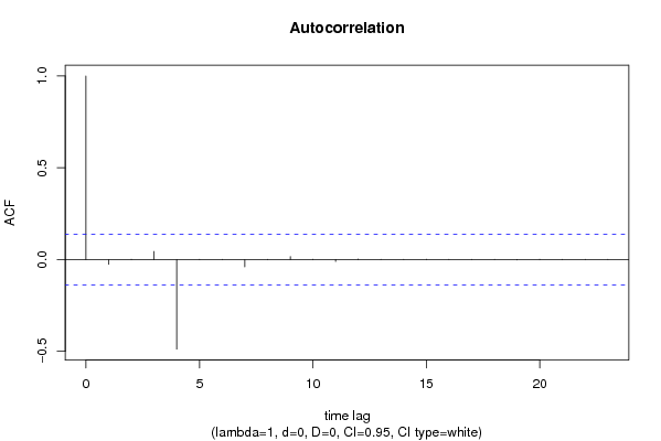
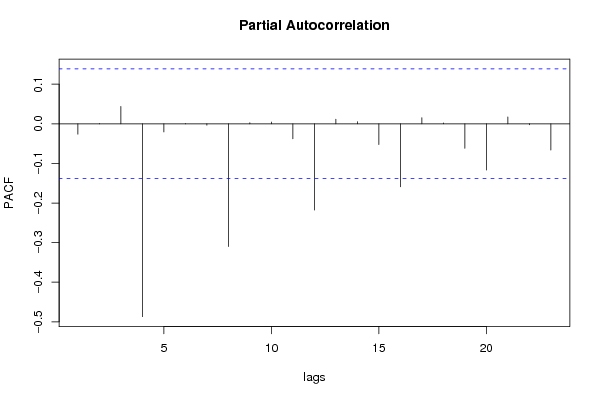
Title produced by software

(Partial) Autocorrelation Function

Date of computation

Tue, 23 Nov 2010 15:03:17 +0000

Cite this page as follows

Statistical Computations at FreeStatistics.org, Office for Research Development and Education, URL https://freestatistics.org/blog/index.php?v=date/2010/Nov/23/t1290524565kgpjp75rblndyci.htm/, Retrieved Sat, 20 Apr 2024 12:39:29 +0000

Statistical Computations at FreeStatistics.org, Office for Research Development and Education, URL https://freestatistics.org/blog/index.php?pk=99221, Retrieved Sat, 20 Apr 2024 12:39:29 +0000

QR Codes:

Paste this QR Code to cite your computation.

Original text written by user:

IsPrivate?

No (this computation is public)

User-defined keywords

Estimated Impact

Family? (F = Feedback message, R = changed R code, M = changed R Module, P = changed Parameters, D = changed Data)

-       [(Partial) Autocorrelation Function] [TIN autocorrelation] [2010-11-23 15:03:17] [f76239c595e4d455b3b05a43389f68d5] [Current]

Feedback Forum

Post a new message

Dataseries X:

Download CSV

Histogram

Boxplots

0.0017356093451131
-3.3306690738755E-14
-3.3306690738755E-14
-3.3306690738755E-14
-3.3306690738755E-14
-0.0028943580263334
3.1086244689504E-14
0.0028943580263312
-3.3306690738755E-14
-3.3306690738755E-14
-3.3306690738755E-14
-3.3306690738755E-14
-0.00057820180853341
8.8817841970013E-16
-0.0023161562177991
3.1086244689504E-14
3.1086244689504E-14
0.0023161562178311
-0.0023161562177991
3.1086244689504E-14
3.1086244689504E-14
3.1086244689504E-14
3.1086244689504E-14
3.1086244689504E-14
0.0028943580263312
-3.3306690738755E-14
-0.0028943580263334
3.1086244689504E-14
0.0028943580263312
-3.3306690738755E-14
-3.3306690738755E-14
-3.3306690738755E-14
-3.3306690738755E-14
-3.3306690738755E-14
-3.3306690738755E-14
-3.3306690738755E-14
-3.3306690738755E-14
-3.3306690738755E-14
-3.3306690738755E-14
-3.3306690738755E-14
-3.3306690738755E-14
-0.0028943580263334
3.1086244689504E-14
3.1086244689504E-14
3.1086244689504E-14
3.1086244689504E-14
3.1086244689504E-14
3.1086244689504E-14
0.0028943580263312
-0.0028943580263334
3.1086244689504E-14
0.0028943580263312
-3.3306690738755E-14
-3.3306690738755E-14
-3.3306690738755E-14
-0.0028943580263334
3.1086244689504E-14
-0.0063972303077691
-3.3750779948605E-14
-3.3750779948605E-14
-0.018251904966934
-1.4654943925052E-14
-0.050574285962915
0.050574285962919
-0.010752791776214
4.7517545453957E-14
4.7517545453957E-14
4.7517545453957E-14
4.7517545453957E-14
0.010752791776247
-0.010752791776214
4.7517545453957E-14
4.7517545453957E-14
0.010752791776247
-0.010752791776214
4.7517545453957E-14
0.010752791776247
-0.010752791776214
4.7517545453957E-14
0.010752791776247
-1.4654943925052E-14
-1.4654943925052E-14
-0.010752791776214
0.010752791776247
-0.010752791776214
4.7517545453957E-14
4.7517545453957E-14
4.7517545453957E-14
4.7517545453957E-14
4.7517545453957E-14
0.010752791776247
-0.010752791776214
4.7517545453957E-14
4.7517545453957E-14
0.010752791776247
-0.010752791776214
0.010752791776247
-1.4654943925052E-14
-0.010752791776214
4.7517545453957E-14
4.7517545453957E-14
4.7517545453957E-14
4.7517545453957E-14
4.7517545453957E-14
0.010752791776247
-1.4654943925052E-14
-1.4654943925052E-14
-0.010752791776214
4.7517545453957E-14
0.010752791776247
-1.4654943925052E-14
-0.0059594932040148
-0.035902852156933
-0.011215070820103
3.7303493627405E-14
3.7303493627405E-14
3.7303493627405E-14
3.7303493627405E-14
3.7303493627405E-14
3.7303493627405E-14
3.7303493627405E-14
3.7303493627405E-14
3.7303493627405E-14
3.7303493627405E-14
3.7303493627405E-14
0.011215070820137
-2.6645352591004E-15
-0.011215070820103
3.7303493627405E-14
3.7303493627405E-14
3.7303493627405E-14
0.011215070820137
-2.6645352591004E-15
-2.6645352591004E-15
-0.011215070820103
0.011215070820137
-2.6645352591004E-15
-2.6645352591004E-15
-0.011215070820103
3.7303493627405E-14
3.7303493627405E-14
3.7303493627405E-14
3.7303493627405E-14
0.011215070820137
-2.6645352591004E-15
-0.011215070820103
3.7303493627405E-14
3.7303493627405E-14
3.7303493627405E-14
3.7303493627405E-14
0.011215070820137
-2.6645352591004E-15
-2.6645352591004E-15
-2.6645352591004E-15
-2.6645352591004E-15
-2.6645352591004E-15
-2.6645352591004E-15
-2.6645352591004E-15
-2.6645352591004E-15
-2.6645352591004E-15
-2.6645352591004E-15
-0.011215070820103
0.011215070820137
-2.6645352591004E-15
-2.6645352591004E-15
-2.6645352591004E-15
-2.6645352591004E-15
-2.6645352591004E-15
-2.6645352591004E-15
-2.6645352591004E-15
-2.6645352591004E-15
-2.6645352591004E-15
-2.6645352591004E-15
-2.6645352591004E-15
-2.6645352591004E-15
-2.6645352591004E-15
-2.6645352591004E-15
-2.6645352591004E-15
-2.6645352591004E-15
-2.6645352591004E-15
-2.6645352591004E-15
-2.6645352591004E-15
-2.6645352591004E-15
-0.011215070820103
3.7303493627405E-14
3.7303493627405E-14
3.7303493627405E-14
-0.062035390919463
0.02566774674859
1.1990408665952E-14
-0.65427640617099
-3.5527136788005E-14
-3.5527136788005E-14
-3.5527136788005E-14
0.65427640617096
-0.025667746748588
0.02566774674859
1.1990408665952E-14
1.1990408665952E-14
-0.025667746748588

Summary of computational transaction
Raw Input	view raw input (R code)
Raw Output	view raw output of R engine
Computing time	2 seconds
R Server	'Sir Ronald Aylmer Fisher' @ 193.190.124.24

\begin{tabular}{lllllllll}
\hline
Summary of computational transaction \tabularnewline
Raw Input & view raw input (R code)  \tabularnewline
Raw Output & view raw output of R engine  \tabularnewline
Computing time & 2 seconds \tabularnewline
R Server & 'Sir Ronald Aylmer Fisher' @ 193.190.124.24 \tabularnewline
\hline
\end{tabular}
%Source: https://freestatistics.org/blog/index.php?pk=99221&T=0

[TABLE]
[ROW][C]Summary of computational transaction[/C][/ROW]
[ROW][C]Raw Input[/C][C]view raw input (R code) [/C][/ROW]
[ROW][C]Raw Output[/C][C]view raw output of R engine [/C][/ROW]
[ROW][C]Computing time[/C][C]2 seconds[/C][/ROW]
[ROW][C]R Server[/C][C]'Sir Ronald Aylmer Fisher' @ 193.190.124.24[/C][/ROW]
[/TABLE]
Source: https://freestatistics.org/blog/index.php?pk=99221&T=0

Globally Unique Identifier (entire table): ba.freestatistics.org/blog/index.php?pk=99221&T=0

As an alternative you can also use a QR Code:

The GUIDs for individual cells are displayed in the table below:

Summary of computational transaction
Raw Input	view raw input (R code)
Raw Output	view raw output of R engine
Computing time	2 seconds
R Server	'Sir Ronald Aylmer Fisher' @ 193.190.124.24

Autocorrelation Function
Time lag k	ACF(k)	T-STAT	P-value
1	-0.026108	-0.3692	0.356175
2	0.001019	0.0144	0.49426
3	0.043971	0.6218	0.267376
4	-0.487984	-6.9011	0
5	-0.000381	-0.0054	0.497855
6	-0.000372	-0.0053	0.497907
7	-0.039317	-0.556	0.289406
8	0.001605	0.0227	0.490957
9	0.015684	0.2218	0.412348
10	0.00126	0.0178	0.492903
11	-0.010465	-0.148	0.441249
12	0.002282	0.0323	0.487146
13	-0.000459	-0.0065	0.497414
14	-0.00057	-0.0081	0.49679
15	0.001205	0.017	0.493211
16	0.000263	0.0037	0.498521
17	-0.000159	-0.0022	0.499104
18	-0.000518	-0.0073	0.497081
19	-0.001657	-0.0234	0.490661
20	0.001091	0.0154	0.49385
21	0.000203	0.0029	0.498856
22	0.000194	0.0027	0.498906
23	-0.00067	-0.0095	0.496224

\begin{tabular}{lllllllll}
\hline
Autocorrelation Function \tabularnewline
Time lag k & ACF(k) & T-STAT & P-value \tabularnewline
1 & -0.026108 & -0.3692 & 0.356175 \tabularnewline
2 & 0.001019 & 0.0144 & 0.49426 \tabularnewline
3 & 0.043971 & 0.6218 & 0.267376 \tabularnewline
4 & -0.487984 & -6.9011 & 0 \tabularnewline
5 & -0.000381 & -0.0054 & 0.497855 \tabularnewline
6 & -0.000372 & -0.0053 & 0.497907 \tabularnewline
7 & -0.039317 & -0.556 & 0.289406 \tabularnewline
8 & 0.001605 & 0.0227 & 0.490957 \tabularnewline
9 & 0.015684 & 0.2218 & 0.412348 \tabularnewline
10 & 0.00126 & 0.0178 & 0.492903 \tabularnewline
11 & -0.010465 & -0.148 & 0.441249 \tabularnewline
12 & 0.002282 & 0.0323 & 0.487146 \tabularnewline
13 & -0.000459 & -0.0065 & 0.497414 \tabularnewline
14 & -0.00057 & -0.0081 & 0.49679 \tabularnewline
15 & 0.001205 & 0.017 & 0.493211 \tabularnewline
16 & 0.000263 & 0.0037 & 0.498521 \tabularnewline
17 & -0.000159 & -0.0022 & 0.499104 \tabularnewline
18 & -0.000518 & -0.0073 & 0.497081 \tabularnewline
19 & -0.001657 & -0.0234 & 0.490661 \tabularnewline
20 & 0.001091 & 0.0154 & 0.49385 \tabularnewline
21 & 0.000203 & 0.0029 & 0.498856 \tabularnewline
22 & 0.000194 & 0.0027 & 0.498906 \tabularnewline
23 & -0.00067 & -0.0095 & 0.496224 \tabularnewline
\hline
\end{tabular}
%Source: https://freestatistics.org/blog/index.php?pk=99221&T=1

[TABLE]
[ROW][C]Autocorrelation Function[/C][/ROW]
[ROW][C]Time lag k[/C][C]ACF(k)[/C][C]T-STAT[/C][C]P-value[/C][/ROW]
[ROW][C]1[/C][C]-0.026108[/C][C]-0.3692[/C][C]0.356175[/C][/ROW]
[ROW][C]2[/C][C]0.001019[/C][C]0.0144[/C][C]0.49426[/C][/ROW]
[ROW][C]3[/C][C]0.043971[/C][C]0.6218[/C][C]0.267376[/C][/ROW]
[ROW][C]4[/C][C]-0.487984[/C][C]-6.9011[/C][C]0[/C][/ROW]
[ROW][C]5[/C][C]-0.000381[/C][C]-0.0054[/C][C]0.497855[/C][/ROW]
[ROW][C]6[/C][C]-0.000372[/C][C]-0.0053[/C][C]0.497907[/C][/ROW]
[ROW][C]7[/C][C]-0.039317[/C][C]-0.556[/C][C]0.289406[/C][/ROW]
[ROW][C]8[/C][C]0.001605[/C][C]0.0227[/C][C]0.490957[/C][/ROW]
[ROW][C]9[/C][C]0.015684[/C][C]0.2218[/C][C]0.412348[/C][/ROW]
[ROW][C]10[/C][C]0.00126[/C][C]0.0178[/C][C]0.492903[/C][/ROW]
[ROW][C]11[/C][C]-0.010465[/C][C]-0.148[/C][C]0.441249[/C][/ROW]
[ROW][C]12[/C][C]0.002282[/C][C]0.0323[/C][C]0.487146[/C][/ROW]
[ROW][C]13[/C][C]-0.000459[/C][C]-0.0065[/C][C]0.497414[/C][/ROW]
[ROW][C]14[/C][C]-0.00057[/C][C]-0.0081[/C][C]0.49679[/C][/ROW]
[ROW][C]15[/C][C]0.001205[/C][C]0.017[/C][C]0.493211[/C][/ROW]
[ROW][C]16[/C][C]0.000263[/C][C]0.0037[/C][C]0.498521[/C][/ROW]
[ROW][C]17[/C][C]-0.000159[/C][C]-0.0022[/C][C]0.499104[/C][/ROW]
[ROW][C]18[/C][C]-0.000518[/C][C]-0.0073[/C][C]0.497081[/C][/ROW]
[ROW][C]19[/C][C]-0.001657[/C][C]-0.0234[/C][C]0.490661[/C][/ROW]
[ROW][C]20[/C][C]0.001091[/C][C]0.0154[/C][C]0.49385[/C][/ROW]
[ROW][C]21[/C][C]0.000203[/C][C]0.0029[/C][C]0.498856[/C][/ROW]
[ROW][C]22[/C][C]0.000194[/C][C]0.0027[/C][C]0.498906[/C][/ROW]
[ROW][C]23[/C][C]-0.00067[/C][C]-0.0095[/C][C]0.496224[/C][/ROW]
[/TABLE]
Source: https://freestatistics.org/blog/index.php?pk=99221&T=1

Globally Unique Identifier (entire table): ba.freestatistics.org/blog/index.php?pk=99221&T=1

As an alternative you can also use a QR Code:

The GUIDs for individual cells are displayed in the table below:

Autocorrelation Function
Time lag k	ACF(k)	T-STAT	P-value
1	-0.026108	-0.3692	0.356175
2	0.001019	0.0144	0.49426
3	0.043971	0.6218	0.267376
4	-0.487984	-6.9011	0
5	-0.000381	-0.0054	0.497855
6	-0.000372	-0.0053	0.497907
7	-0.039317	-0.556	0.289406
8	0.001605	0.0227	0.490957
9	0.015684	0.2218	0.412348
10	0.00126	0.0178	0.492903
11	-0.010465	-0.148	0.441249
12	0.002282	0.0323	0.487146
13	-0.000459	-0.0065	0.497414
14	-0.00057	-0.0081	0.49679
15	0.001205	0.017	0.493211
16	0.000263	0.0037	0.498521
17	-0.000159	-0.0022	0.499104
18	-0.000518	-0.0073	0.497081
19	-0.001657	-0.0234	0.490661
20	0.001091	0.0154	0.49385
21	0.000203	0.0029	0.498856
22	0.000194	0.0027	0.498906
23	-0.00067	-0.0095	0.496224

Partial Autocorrelation Function
Time lag k	PACF(k)	T-STAT	P-value
1	-0.026108	-0.3692	0.356175
2	0.000337	0.0048	0.498099
3	0.044037	0.6228	0.267072
4	-0.486964	-6.8867	0
5	-0.020375	-0.2881	0.386768
6	-0.000528	-0.0075	0.497023
7	-0.003398	-0.0481	0.480858
8	-0.310007	-4.3842	9e-06
9	0.002949	0.0417	0.48339
10	0.004327	0.0612	0.475636
11	-0.037538	-0.5309	0.298052
12	-0.21758	-3.077	0.001192
13	0.011628	0.1644	0.434774
14	0.005488	0.0776	0.469107
15	-0.052117	-0.737	0.23098
16	-0.159019	-2.2489	0.012806
17	0.015284	0.2161	0.414549
18	0.00207	0.0293	0.488337
19	-0.061563	-0.8706	0.192501
20	-0.116636	-1.6495	0.050309
21	0.017178	0.2429	0.404155
22	-0.002334	-0.033	0.486849
23	-0.066099	-0.9348	0.175514

\begin{tabular}{lllllllll}
\hline
Partial Autocorrelation Function \tabularnewline
Time lag k & PACF(k) & T-STAT & P-value \tabularnewline
1 & -0.026108 & -0.3692 & 0.356175 \tabularnewline
2 & 0.000337 & 0.0048 & 0.498099 \tabularnewline
3 & 0.044037 & 0.6228 & 0.267072 \tabularnewline
4 & -0.486964 & -6.8867 & 0 \tabularnewline
5 & -0.020375 & -0.2881 & 0.386768 \tabularnewline
6 & -0.000528 & -0.0075 & 0.497023 \tabularnewline
7 & -0.003398 & -0.0481 & 0.480858 \tabularnewline
8 & -0.310007 & -4.3842 & 9e-06 \tabularnewline
9 & 0.002949 & 0.0417 & 0.48339 \tabularnewline
10 & 0.004327 & 0.0612 & 0.475636 \tabularnewline
11 & -0.037538 & -0.5309 & 0.298052 \tabularnewline
12 & -0.21758 & -3.077 & 0.001192 \tabularnewline
13 & 0.011628 & 0.1644 & 0.434774 \tabularnewline
14 & 0.005488 & 0.0776 & 0.469107 \tabularnewline
15 & -0.052117 & -0.737 & 0.23098 \tabularnewline
16 & -0.159019 & -2.2489 & 0.012806 \tabularnewline
17 & 0.015284 & 0.2161 & 0.414549 \tabularnewline
18 & 0.00207 & 0.0293 & 0.488337 \tabularnewline
19 & -0.061563 & -0.8706 & 0.192501 \tabularnewline
20 & -0.116636 & -1.6495 & 0.050309 \tabularnewline
21 & 0.017178 & 0.2429 & 0.404155 \tabularnewline
22 & -0.002334 & -0.033 & 0.486849 \tabularnewline
23 & -0.066099 & -0.9348 & 0.175514 \tabularnewline
\hline
\end{tabular}
%Source: https://freestatistics.org/blog/index.php?pk=99221&T=2

[TABLE]
[ROW][C]Partial Autocorrelation Function[/C][/ROW]
[ROW][C]Time lag k[/C][C]PACF(k)[/C][C]T-STAT[/C][C]P-value[/C][/ROW]
[ROW][C]1[/C][C]-0.026108[/C][C]-0.3692[/C][C]0.356175[/C][/ROW]
[ROW][C]2[/C][C]0.000337[/C][C]0.0048[/C][C]0.498099[/C][/ROW]
[ROW][C]3[/C][C]0.044037[/C][C]0.6228[/C][C]0.267072[/C][/ROW]
[ROW][C]4[/C][C]-0.486964[/C][C]-6.8867[/C][C]0[/C][/ROW]
[ROW][C]5[/C][C]-0.020375[/C][C]-0.2881[/C][C]0.386768[/C][/ROW]
[ROW][C]6[/C][C]-0.000528[/C][C]-0.0075[/C][C]0.497023[/C][/ROW]
[ROW][C]7[/C][C]-0.003398[/C][C]-0.0481[/C][C]0.480858[/C][/ROW]
[ROW][C]8[/C][C]-0.310007[/C][C]-4.3842[/C][C]9e-06[/C][/ROW]
[ROW][C]9[/C][C]0.002949[/C][C]0.0417[/C][C]0.48339[/C][/ROW]
[ROW][C]10[/C][C]0.004327[/C][C]0.0612[/C][C]0.475636[/C][/ROW]
[ROW][C]11[/C][C]-0.037538[/C][C]-0.5309[/C][C]0.298052[/C][/ROW]
[ROW][C]12[/C][C]-0.21758[/C][C]-3.077[/C][C]0.001192[/C][/ROW]
[ROW][C]13[/C][C]0.011628[/C][C]0.1644[/C][C]0.434774[/C][/ROW]
[ROW][C]14[/C][C]0.005488[/C][C]0.0776[/C][C]0.469107[/C][/ROW]
[ROW][C]15[/C][C]-0.052117[/C][C]-0.737[/C][C]0.23098[/C][/ROW]
[ROW][C]16[/C][C]-0.159019[/C][C]-2.2489[/C][C]0.012806[/C][/ROW]
[ROW][C]17[/C][C]0.015284[/C][C]0.2161[/C][C]0.414549[/C][/ROW]
[ROW][C]18[/C][C]0.00207[/C][C]0.0293[/C][C]0.488337[/C][/ROW]
[ROW][C]19[/C][C]-0.061563[/C][C]-0.8706[/C][C]0.192501[/C][/ROW]
[ROW][C]20[/C][C]-0.116636[/C][C]-1.6495[/C][C]0.050309[/C][/ROW]
[ROW][C]21[/C][C]0.017178[/C][C]0.2429[/C][C]0.404155[/C][/ROW]
[ROW][C]22[/C][C]-0.002334[/C][C]-0.033[/C][C]0.486849[/C][/ROW]
[ROW][C]23[/C][C]-0.066099[/C][C]-0.9348[/C][C]0.175514[/C][/ROW]
[/TABLE]
Source: https://freestatistics.org/blog/index.php?pk=99221&T=2

Globally Unique Identifier (entire table): ba.freestatistics.org/blog/index.php?pk=99221&T=2

As an alternative you can also use a QR Code:

The GUIDs for individual cells are displayed in the table below:

Partial Autocorrelation Function
Time lag k	PACF(k)	T-STAT	P-value
1	-0.026108	-0.3692	0.356175
2	0.000337	0.0048	0.498099
3	0.044037	0.6228	0.267072
4	-0.486964	-6.8867	0
5	-0.020375	-0.2881	0.386768
6	-0.000528	-0.0075	0.497023
7	-0.003398	-0.0481	0.480858
8	-0.310007	-4.3842	9e-06
9	0.002949	0.0417	0.48339
10	0.004327	0.0612	0.475636
11	-0.037538	-0.5309	0.298052
12	-0.21758	-3.077	0.001192
13	0.011628	0.1644	0.434774
14	0.005488	0.0776	0.469107
15	-0.052117	-0.737	0.23098
16	-0.159019	-2.2489	0.012806
17	0.015284	0.2161	0.414549
18	0.00207	0.0293	0.488337
19	-0.061563	-0.8706	0.192501
20	-0.116636	-1.6495	0.050309
21	0.017178	0.2429	0.404155
22	-0.002334	-0.033	0.486849
23	-0.066099	-0.9348	0.175514

Figure 1

PNG link

Postscript link

PDF link

Figure 2

PNG link

Postscript link

PDF link

Parameters (Session):

par1 = Default ; par2 = 1 ; par3 = 0 ; par4 = 0 ; par5 = 12 ; par6 = White Noise ; par7 = 0.95 ;

Parameters (R input):

par1 = Default ; par2 = 1 ; par3 = 0 ; par4 = 0 ; par5 = 12 ; par6 = White Noise ; par7 = 0.95 ;

R code (references can be found in the software module):

if (par1 == 'Default') {
par1 = 10*log10(length(x))
} else {
par1 <- as.numeric(par1)
}
par2 <- as.numeric(par2)
par3 <- as.numeric(par3)
par4 <- as.numeric(par4)
par5 <- as.numeric(par5)
if (par6 == 'White Noise') par6 <- 'white' else par6 <- 'ma'
par7 <- as.numeric(par7)
if (par2 == 0) {
x <- log(x)
} else {
x <- (x ^ par2 - 1) / par2
}
if (par3 > 0) x <- diff(x,lag=1,difference=par3)
if (par4 > 0) x <- diff(x,lag=par5,difference=par4)
bitmap(file='pic1.png')
racf <- acf(x, par1, main='Autocorrelation', xlab='time lag', ylab='ACF', ci.type=par6, ci=par7, sub=paste('(lambda=',par2,', d=',par3,', D=',par4,', CI=', par7, ', CI type=',par6,')',sep=''))
dev.off()
bitmap(file='pic2.png')
rpacf <- pacf(x,par1,main='Partial Autocorrelation',xlab='lags',ylab='PACF')
dev.off()
(myacf <- c(racf$acf))
(mypacf <- c(rpacf$acf))
lengthx <- length(x)
sqrtn <- sqrt(lengthx)
load(file='createtable')
a<-table.start()
a<-table.row.start(a)
a<-table.element(a,'Autocorrelation Function',4,TRUE)
a<-table.row.end(a)
a<-table.row.start(a)
a<-table.element(a,'Time lag k',header=TRUE)
a<-table.element(a,hyperlink('basics.htm','ACF(k)','click here for more information about the Autocorrelation Function'),header=TRUE)
a<-table.element(a,'T-STAT',header=TRUE)
a<-table.element(a,'P-value',header=TRUE)
a<-table.row.end(a)
for (i in 2:(par1+1)) {
a<-table.row.start(a)
a<-table.element(a,i-1,header=TRUE)
a<-table.element(a,round(myacf[i],6))
mytstat <- myacf[i]*sqrtn
a<-table.element(a,round(mytstat,4))
a<-table.element(a,round(1-pt(abs(mytstat),lengthx),6))
a<-table.row.end(a)
}
a<-table.end(a)
table.save(a,file='mytable.tab')
a<-table.start()
a<-table.row.start(a)
a<-table.element(a,'Partial Autocorrelation Function',4,TRUE)
a<-table.row.end(a)
a<-table.row.start(a)
a<-table.element(a,'Time lag k',header=TRUE)
a<-table.element(a,hyperlink('basics.htm','PACF(k)','click here for more information about the Partial Autocorrelation Function'),header=TRUE)
a<-table.element(a,'T-STAT',header=TRUE)
a<-table.element(a,'P-value',header=TRUE)
a<-table.row.end(a)
for (i in 1:par1) {
a<-table.row.start(a)
a<-table.element(a,i,header=TRUE)
a<-table.element(a,round(mypacf[i],6))
mytstat <- mypacf[i]*sqrtn
a<-table.element(a,round(mytstat,4))
a<-table.element(a,round(1-pt(abs(mytstat),lengthx),6))
a<-table.row.end(a)
}
a<-table.end(a)
table.save(a,file='mytable1.tab')

Free Statistics

Description of Statistical Computation

Tree of Dependent Computations

Dataset

Tables (Output of Computation)

Figures (Output of Computation)

Input Parameters & R Code