Repository of Reproducible Computations

Free Statistics

of Irreproducible Research!

Author's title

Author

*The author of this computation has been verified*

R Software Module

rwasp_autocorrelation.wasp

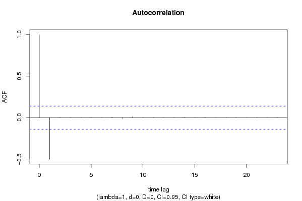
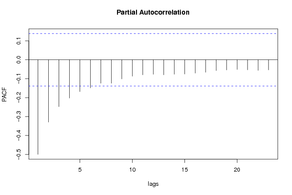
Title produced by software

(Partial) Autocorrelation Function

Date of computation

Tue, 23 Nov 2010 14:45:35 +0000

Cite this page as follows

Statistical Computations at FreeStatistics.org, Office for Research Development and Education, URL https://freestatistics.org/blog/index.php?v=date/2010/Nov/23/t1290523494mrvuf8pmx3fs8hn.htm/, Retrieved Thu, 25 Apr 2024 01:41:04 +0000

Statistical Computations at FreeStatistics.org, Office for Research Development and Education, URL https://freestatistics.org/blog/index.php?pk=99177, Retrieved Thu, 25 Apr 2024 01:41:04 +0000

QR Codes:

Paste this QR Code to cite your computation.

Original text written by user:

IsPrivate?

No (this computation is public)

User-defined keywords

beursspel test

Estimated Impact

117

Family? (F = Feedback message, R = changed R code, M = changed R Module, P = changed Parameters, D = changed Data)

-       [(Partial) Autocorrelation Function] [autocorrelation t...] [2010-11-23 14:45:35] [f76239c595e4d455b3b05a43389f68d5] [Current]

Feedback Forum

Post a new message

Dataseries X:

Download CSV

Histogram

Boxplots

-0.0042361726044575
-4.3964831775156E-14
0.0042361726044557
-0.0042361726044575
0.0042361726044557
4.2188474935756E-14
4.2188474935756E-14
4.2188474935756E-14
4.2188474935756E-14
-0.0042361726044575
0.0042361726044557
4.2188474935756E-14
4.2188474935756E-14
-0.0042361726044575
-4.3964831775156E-14
-4.3964831775156E-14
-4.3964831775156E-14
-4.3964831775156E-14
-4.3964831775156E-14
0.0042361726044557
4.2188474935756E-14
4.2188474935756E-14
-0.0042361726044575
-4.3964831775156E-14
0.0042361726044557
-0.0042361726044575
-4.3964831775156E-14
-4.3964831775156E-14
-4.3964831775156E-14
0.0042361726044557
-0.0042361726044575
-4.3964831775156E-14
-4.3964831775156E-14
-4.3964831775156E-14
-4.3964831775156E-14
0.0042361726044557
4.2188474935756E-14
-0.0042361726044575
-4.3964831775156E-14
-4.3964831775156E-14
0.0052924177514559
-0.0052924177515092
0.0052924177514559
-9.3258734068513E-15
-9.3258734068513E-15
-0.0052924177515092
-4.3964831775156E-14
-4.3964831775156E-14
-4.3964831775156E-14
-4.3964831775156E-14
0.0052924177514559
-9.3258734068513E-15
-9.3258734068513E-15
-9.3258734068513E-15
-9.3258734068513E-15
-0.0052924177515092
0.0052924177514559
-9.3258734068513E-15
-9.3258734068513E-15
-9.3258734068513E-15
-0.0052924177515092
0.0052924177514559
-0.0052924177515092
-4.3964831775156E-14
-4.3964831775156E-14
0.0052924177514559
-9.3258734068513E-15
-0.0052924177515092
-4.3964831775156E-14
0.0052924177514559
-9.3258734068513E-15
-9.3258734068513E-15
-0.0052924177515092
-4.3964831775156E-14
0.0015906684159561
-3.3306690738755E-14
-0.0053120974849334
0.0053120974848566
-3.3306690738755E-14
-3.3306690738755E-14
-3.3306690738755E-14
-3.3306690738755E-14
-3.3306690738755E-14
-3.3306690738755E-14
-0.0053120974849334
-4.3520742565306E-14
0.0053120974848566
-3.3306690738755E-14
-3.3306690738755E-14
-3.3306690738755E-14
-3.3306690738755E-14
-3.3306690738755E-14
-3.3306690738755E-14
-3.3306690738755E-14
-3.3306690738755E-14
-0.0053120974849334
-4.3520742565306E-14
-4.3520742565306E-14
-4.3520742565306E-14
-0.0093646169310437
0.014676714415899
-0.0053120974849334
0.0053120974848566
-3.3306690738755E-14
-3.3306690738755E-14
-3.3306690738755E-14
-0.0053120974849334
0.0013306721856563
-0.91895384929365
0.91895384929359
-4.8849813083507E-14
-4.8849813083507E-14
-4.8849813083507E-14
-0.0047987295499485
-4.3520742565306E-14
-4.3520742565306E-14
-4.3520742565306E-14
-4.3520742565306E-14
-4.3520742565306E-14
0.0047987295498562
-4.8849813083507E-14
-0.0026631174194489
-0.013423020332165
-0.0029774010356243
-0.0048913140998841
-4.3076653355456E-14
-4.3076653355456E-14
0.004891314099857
1.5987211554602E-14
1.5987211554602E-14
-0.0048913140998841
-4.3076653355456E-14
-4.3076653355456E-14
-4.3076653355456E-14
-4.3076653355456E-14
-4.3076653355456E-14
0.004891314099857
1.5987211554602E-14
-0.0048913140998841
0.004891314099857
1.5987211554602E-14
1.5987211554602E-14
1.5987211554602E-14
1.5987211554602E-14
-0.0048913140998841
0.004891314099857
1.5987211554602E-14
1.5987211554602E-14
-0.0048913140998841
0.004891314099857
-0.0048913140998841
-4.3076653355456E-14
-4.3076653355456E-14
-4.3076653355456E-14
-4.3076653355456E-14
-4.3076653355456E-14
-4.3076653355456E-14
-4.3076653355456E-14
-4.3076653355456E-14
-4.3076653355456E-14
-4.3076653355456E-14
-4.3076653355456E-14
-4.3076653355456E-14
-4.3076653355456E-14
-4.3076653355456E-14
-4.3076653355456E-14
-4.3076653355456E-14
-4.3076653355456E-14
0.004891314099857
-0.0048913140998841
-4.3076653355456E-14
0.004891314099857
1.5987211554602E-14
-0.0048913140998841
-4.3076653355456E-14
0.004891314099857
-0.0048913140998841
-4.3076653355456E-14
-4.3076653355456E-14
-4.3076653355456E-14
-4.3076653355456E-14
0.004891314099857
1.5987211554602E-14
-0.0048913140998841
-4.3076653355456E-14
0.004891314099857
1.5987211554602E-14
1.5987211554602E-14
1.5987211554602E-14
1.5987211554602E-14
-0.0048913140998841
-0.018974857760943
-1.0214051826551E-14
-1.0214051826551E-14
-1.0214051826551E-14
0.02684357289639
-2.4424906541753E-14
-0.026843572896424
-1.0214051826551E-14
0.02684357289639

Summary of computational transaction
Raw Input	view raw input (R code)
Raw Output	view raw output of R engine
Computing time	2 seconds
R Server	'RServer@AstonUniversity' @ vre.aston.ac.uk

\begin{tabular}{lllllllll}
\hline
Summary of computational transaction \tabularnewline
Raw Input & view raw input (R code)  \tabularnewline
Raw Output & view raw output of R engine  \tabularnewline
Computing time & 2 seconds \tabularnewline
R Server & 'RServer@AstonUniversity' @ vre.aston.ac.uk \tabularnewline
\hline
\end{tabular}
%Source: https://freestatistics.org/blog/index.php?pk=99177&T=0

[TABLE]
[ROW][C]Summary of computational transaction[/C][/ROW]
[ROW][C]Raw Input[/C][C]view raw input (R code) [/C][/ROW]
[ROW][C]Raw Output[/C][C]view raw output of R engine [/C][/ROW]
[ROW][C]Computing time[/C][C]2 seconds[/C][/ROW]
[ROW][C]R Server[/C][C]'RServer@AstonUniversity' @ vre.aston.ac.uk[/C][/ROW]
[/TABLE]
Source: https://freestatistics.org/blog/index.php?pk=99177&T=0

Globally Unique Identifier (entire table): ba.freestatistics.org/blog/index.php?pk=99177&T=0

As an alternative you can also use a QR Code:

The GUIDs for individual cells are displayed in the table below:

Summary of computational transaction
Raw Input	view raw input (R code)
Raw Output	view raw output of R engine
Computing time	2 seconds
R Server	'RServer@AstonUniversity' @ vre.aston.ac.uk

Autocorrelation Function
Time lag k	ACF(k)	T-STAT	P-value
1	-0.499686	-7.0666	0
2	0.002744	0.0388	0.484544
3	-0.003002	-0.0425	0.48309
4	-0.002362	-0.0334	0.486693
5	0.002345	0.0332	0.486786
6	-0.002703	-0.0382	0.484775
7	0.005884	0.0832	0.466885
8	-0.010996	-0.1555	0.438289
9	0.01301	0.184	0.427102
10	-0.002436	-0.0345	0.486275
11	-0.002674	-0.0378	0.484934
12	-0.001596	-0.0226	0.491008
13	-0.00302	-0.0427	0.482991
14	0.003113	0.044	0.482462
15	-0.001067	-0.0151	0.493986
16	0.002499	0.0353	0.485922
17	7.4e-05	0.0011	0.499581
18	0.002754	0.0389	0.484485
19	-0.002676	-0.0378	0.484926
20	-0.000169	-0.0024	0.499047
21	-0.002492	-0.0352	0.485959
22	-0.000415	-0.0059	0.497659
23	0.00288	0.0407	0.483775

\begin{tabular}{lllllllll}
\hline
Autocorrelation Function \tabularnewline
Time lag k & ACF(k) & T-STAT & P-value \tabularnewline
1 & -0.499686 & -7.0666 & 0 \tabularnewline
2 & 0.002744 & 0.0388 & 0.484544 \tabularnewline
3 & -0.003002 & -0.0425 & 0.48309 \tabularnewline
4 & -0.002362 & -0.0334 & 0.486693 \tabularnewline
5 & 0.002345 & 0.0332 & 0.486786 \tabularnewline
6 & -0.002703 & -0.0382 & 0.484775 \tabularnewline
7 & 0.005884 & 0.0832 & 0.466885 \tabularnewline
8 & -0.010996 & -0.1555 & 0.438289 \tabularnewline
9 & 0.01301 & 0.184 & 0.427102 \tabularnewline
10 & -0.002436 & -0.0345 & 0.486275 \tabularnewline
11 & -0.002674 & -0.0378 & 0.484934 \tabularnewline
12 & -0.001596 & -0.0226 & 0.491008 \tabularnewline
13 & -0.00302 & -0.0427 & 0.482991 \tabularnewline
14 & 0.003113 & 0.044 & 0.482462 \tabularnewline
15 & -0.001067 & -0.0151 & 0.493986 \tabularnewline
16 & 0.002499 & 0.0353 & 0.485922 \tabularnewline
17 & 7.4e-05 & 0.0011 & 0.499581 \tabularnewline
18 & 0.002754 & 0.0389 & 0.484485 \tabularnewline
19 & -0.002676 & -0.0378 & 0.484926 \tabularnewline
20 & -0.000169 & -0.0024 & 0.499047 \tabularnewline
21 & -0.002492 & -0.0352 & 0.485959 \tabularnewline
22 & -0.000415 & -0.0059 & 0.497659 \tabularnewline
23 & 0.00288 & 0.0407 & 0.483775 \tabularnewline
\hline
\end{tabular}
%Source: https://freestatistics.org/blog/index.php?pk=99177&T=1

[TABLE]
[ROW][C]Autocorrelation Function[/C][/ROW]
[ROW][C]Time lag k[/C][C]ACF(k)[/C][C]T-STAT[/C][C]P-value[/C][/ROW]
[ROW][C]1[/C][C]-0.499686[/C][C]-7.0666[/C][C]0[/C][/ROW]
[ROW][C]2[/C][C]0.002744[/C][C]0.0388[/C][C]0.484544[/C][/ROW]
[ROW][C]3[/C][C]-0.003002[/C][C]-0.0425[/C][C]0.48309[/C][/ROW]
[ROW][C]4[/C][C]-0.002362[/C][C]-0.0334[/C][C]0.486693[/C][/ROW]
[ROW][C]5[/C][C]0.002345[/C][C]0.0332[/C][C]0.486786[/C][/ROW]
[ROW][C]6[/C][C]-0.002703[/C][C]-0.0382[/C][C]0.484775[/C][/ROW]
[ROW][C]7[/C][C]0.005884[/C][C]0.0832[/C][C]0.466885[/C][/ROW]
[ROW][C]8[/C][C]-0.010996[/C][C]-0.1555[/C][C]0.438289[/C][/ROW]
[ROW][C]9[/C][C]0.01301[/C][C]0.184[/C][C]0.427102[/C][/ROW]
[ROW][C]10[/C][C]-0.002436[/C][C]-0.0345[/C][C]0.486275[/C][/ROW]
[ROW][C]11[/C][C]-0.002674[/C][C]-0.0378[/C][C]0.484934[/C][/ROW]
[ROW][C]12[/C][C]-0.001596[/C][C]-0.0226[/C][C]0.491008[/C][/ROW]
[ROW][C]13[/C][C]-0.00302[/C][C]-0.0427[/C][C]0.482991[/C][/ROW]
[ROW][C]14[/C][C]0.003113[/C][C]0.044[/C][C]0.482462[/C][/ROW]
[ROW][C]15[/C][C]-0.001067[/C][C]-0.0151[/C][C]0.493986[/C][/ROW]
[ROW][C]16[/C][C]0.002499[/C][C]0.0353[/C][C]0.485922[/C][/ROW]
[ROW][C]17[/C][C]7.4e-05[/C][C]0.0011[/C][C]0.499581[/C][/ROW]
[ROW][C]18[/C][C]0.002754[/C][C]0.0389[/C][C]0.484485[/C][/ROW]
[ROW][C]19[/C][C]-0.002676[/C][C]-0.0378[/C][C]0.484926[/C][/ROW]
[ROW][C]20[/C][C]-0.000169[/C][C]-0.0024[/C][C]0.499047[/C][/ROW]
[ROW][C]21[/C][C]-0.002492[/C][C]-0.0352[/C][C]0.485959[/C][/ROW]
[ROW][C]22[/C][C]-0.000415[/C][C]-0.0059[/C][C]0.497659[/C][/ROW]
[ROW][C]23[/C][C]0.00288[/C][C]0.0407[/C][C]0.483775[/C][/ROW]
[/TABLE]
Source: https://freestatistics.org/blog/index.php?pk=99177&T=1

Globally Unique Identifier (entire table): ba.freestatistics.org/blog/index.php?pk=99177&T=1

As an alternative you can also use a QR Code:

The GUIDs for individual cells are displayed in the table below:

Autocorrelation Function
Time lag k	ACF(k)	T-STAT	P-value
1	-0.499686	-7.0666	0
2	0.002744	0.0388	0.484544
3	-0.003002	-0.0425	0.48309
4	-0.002362	-0.0334	0.486693
5	0.002345	0.0332	0.486786
6	-0.002703	-0.0382	0.484775
7	0.005884	0.0832	0.466885
8	-0.010996	-0.1555	0.438289
9	0.01301	0.184	0.427102
10	-0.002436	-0.0345	0.486275
11	-0.002674	-0.0378	0.484934
12	-0.001596	-0.0226	0.491008
13	-0.00302	-0.0427	0.482991
14	0.003113	0.044	0.482462
15	-0.001067	-0.0151	0.493986
16	0.002499	0.0353	0.485922
17	7.4e-05	0.0011	0.499581
18	0.002754	0.0389	0.484485
19	-0.002676	-0.0378	0.484926
20	-0.000169	-0.0024	0.499047
21	-0.002492	-0.0352	0.485959
22	-0.000415	-0.0059	0.497659
23	0.00288	0.0407	0.483775

Partial Autocorrelation Function
Time lag k	PACF(k)	T-STAT	P-value
1	-0.499686	-7.0666	0
2	-0.329119	-4.6544	3e-06
3	-0.247572	-3.5012	0.000286
4	-0.202146	-2.8588	0.002352
5	-0.168055	-2.3767	0.009207
6	-0.148395	-2.0986	0.018552
7	-0.123615	-1.7482	0.040983
8	-0.123839	-1.7513	0.04071
9	-0.100945	-1.4276	0.077487
10	-0.086599	-1.2247	0.111066
11	-0.079599	-1.1257	0.130821
12	-0.076513	-1.0821	0.140266
13	-0.079239	-1.1206	0.131899
14	-0.076033	-1.0753	0.141775
15	-0.075238	-1.064	0.144299
16	-0.070373	-0.9952	0.160415
17	-0.065727	-0.9295	0.176871
18	-0.056617	-0.8007	0.21213
19	-0.053503	-0.7566	0.225075
20	-0.050818	-0.7187	0.23659
21	-0.053083	-0.7507	0.226857
22	-0.05584	-0.7897	0.215318
23	-0.053201	-0.7524	0.226354

\begin{tabular}{lllllllll}
\hline
Partial Autocorrelation Function \tabularnewline
Time lag k & PACF(k) & T-STAT & P-value \tabularnewline
1 & -0.499686 & -7.0666 & 0 \tabularnewline
2 & -0.329119 & -4.6544 & 3e-06 \tabularnewline
3 & -0.247572 & -3.5012 & 0.000286 \tabularnewline
4 & -0.202146 & -2.8588 & 0.002352 \tabularnewline
5 & -0.168055 & -2.3767 & 0.009207 \tabularnewline
6 & -0.148395 & -2.0986 & 0.018552 \tabularnewline
7 & -0.123615 & -1.7482 & 0.040983 \tabularnewline
8 & -0.123839 & -1.7513 & 0.04071 \tabularnewline
9 & -0.100945 & -1.4276 & 0.077487 \tabularnewline
10 & -0.086599 & -1.2247 & 0.111066 \tabularnewline
11 & -0.079599 & -1.1257 & 0.130821 \tabularnewline
12 & -0.076513 & -1.0821 & 0.140266 \tabularnewline
13 & -0.079239 & -1.1206 & 0.131899 \tabularnewline
14 & -0.076033 & -1.0753 & 0.141775 \tabularnewline
15 & -0.075238 & -1.064 & 0.144299 \tabularnewline
16 & -0.070373 & -0.9952 & 0.160415 \tabularnewline
17 & -0.065727 & -0.9295 & 0.176871 \tabularnewline
18 & -0.056617 & -0.8007 & 0.21213 \tabularnewline
19 & -0.053503 & -0.7566 & 0.225075 \tabularnewline
20 & -0.050818 & -0.7187 & 0.23659 \tabularnewline
21 & -0.053083 & -0.7507 & 0.226857 \tabularnewline
22 & -0.05584 & -0.7897 & 0.215318 \tabularnewline
23 & -0.053201 & -0.7524 & 0.226354 \tabularnewline
\hline
\end{tabular}
%Source: https://freestatistics.org/blog/index.php?pk=99177&T=2

[TABLE]
[ROW][C]Partial Autocorrelation Function[/C][/ROW]
[ROW][C]Time lag k[/C][C]PACF(k)[/C][C]T-STAT[/C][C]P-value[/C][/ROW]
[ROW][C]1[/C][C]-0.499686[/C][C]-7.0666[/C][C]0[/C][/ROW]
[ROW][C]2[/C][C]-0.329119[/C][C]-4.6544[/C][C]3e-06[/C][/ROW]
[ROW][C]3[/C][C]-0.247572[/C][C]-3.5012[/C][C]0.000286[/C][/ROW]
[ROW][C]4[/C][C]-0.202146[/C][C]-2.8588[/C][C]0.002352[/C][/ROW]
[ROW][C]5[/C][C]-0.168055[/C][C]-2.3767[/C][C]0.009207[/C][/ROW]
[ROW][C]6[/C][C]-0.148395[/C][C]-2.0986[/C][C]0.018552[/C][/ROW]
[ROW][C]7[/C][C]-0.123615[/C][C]-1.7482[/C][C]0.040983[/C][/ROW]
[ROW][C]8[/C][C]-0.123839[/C][C]-1.7513[/C][C]0.04071[/C][/ROW]
[ROW][C]9[/C][C]-0.100945[/C][C]-1.4276[/C][C]0.077487[/C][/ROW]
[ROW][C]10[/C][C]-0.086599[/C][C]-1.2247[/C][C]0.111066[/C][/ROW]
[ROW][C]11[/C][C]-0.079599[/C][C]-1.1257[/C][C]0.130821[/C][/ROW]
[ROW][C]12[/C][C]-0.076513[/C][C]-1.0821[/C][C]0.140266[/C][/ROW]
[ROW][C]13[/C][C]-0.079239[/C][C]-1.1206[/C][C]0.131899[/C][/ROW]
[ROW][C]14[/C][C]-0.076033[/C][C]-1.0753[/C][C]0.141775[/C][/ROW]
[ROW][C]15[/C][C]-0.075238[/C][C]-1.064[/C][C]0.144299[/C][/ROW]
[ROW][C]16[/C][C]-0.070373[/C][C]-0.9952[/C][C]0.160415[/C][/ROW]
[ROW][C]17[/C][C]-0.065727[/C][C]-0.9295[/C][C]0.176871[/C][/ROW]
[ROW][C]18[/C][C]-0.056617[/C][C]-0.8007[/C][C]0.21213[/C][/ROW]
[ROW][C]19[/C][C]-0.053503[/C][C]-0.7566[/C][C]0.225075[/C][/ROW]
[ROW][C]20[/C][C]-0.050818[/C][C]-0.7187[/C][C]0.23659[/C][/ROW]
[ROW][C]21[/C][C]-0.053083[/C][C]-0.7507[/C][C]0.226857[/C][/ROW]
[ROW][C]22[/C][C]-0.05584[/C][C]-0.7897[/C][C]0.215318[/C][/ROW]
[ROW][C]23[/C][C]-0.053201[/C][C]-0.7524[/C][C]0.226354[/C][/ROW]
[/TABLE]
Source: https://freestatistics.org/blog/index.php?pk=99177&T=2

Globally Unique Identifier (entire table): ba.freestatistics.org/blog/index.php?pk=99177&T=2

As an alternative you can also use a QR Code:

The GUIDs for individual cells are displayed in the table below:

Partial Autocorrelation Function
Time lag k	PACF(k)	T-STAT	P-value
1	-0.499686	-7.0666	0
2	-0.329119	-4.6544	3e-06
3	-0.247572	-3.5012	0.000286
4	-0.202146	-2.8588	0.002352
5	-0.168055	-2.3767	0.009207
6	-0.148395	-2.0986	0.018552
7	-0.123615	-1.7482	0.040983
8	-0.123839	-1.7513	0.04071
9	-0.100945	-1.4276	0.077487
10	-0.086599	-1.2247	0.111066
11	-0.079599	-1.1257	0.130821
12	-0.076513	-1.0821	0.140266
13	-0.079239	-1.1206	0.131899
14	-0.076033	-1.0753	0.141775
15	-0.075238	-1.064	0.144299
16	-0.070373	-0.9952	0.160415
17	-0.065727	-0.9295	0.176871
18	-0.056617	-0.8007	0.21213
19	-0.053503	-0.7566	0.225075
20	-0.050818	-0.7187	0.23659
21	-0.053083	-0.7507	0.226857
22	-0.05584	-0.7897	0.215318
23	-0.053201	-0.7524	0.226354

Figure 1

PNG link

Postscript link

PDF link

Figure 2

PNG link

Postscript link

PDF link

Parameters (Session):

par1 = Default ; par2 = 1 ; par3 = 0 ; par4 = 0 ; par5 = 12 ; par6 = White Noise ; par7 = 0.95 ;

Parameters (R input):

par1 = Default ; par2 = 1 ; par3 = 0 ; par4 = 0 ; par5 = 12 ; par6 = White Noise ; par7 = 0.95 ;

R code (references can be found in the software module):

if (par1 == 'Default') {
par1 = 10*log10(length(x))
} else {
par1 <- as.numeric(par1)
}
par2 <- as.numeric(par2)
par3 <- as.numeric(par3)
par4 <- as.numeric(par4)
par5 <- as.numeric(par5)
if (par6 == 'White Noise') par6 <- 'white' else par6 <- 'ma'
par7 <- as.numeric(par7)
if (par2 == 0) {
x <- log(x)
} else {
x <- (x ^ par2 - 1) / par2
}
if (par3 > 0) x <- diff(x,lag=1,difference=par3)
if (par4 > 0) x <- diff(x,lag=par5,difference=par4)
bitmap(file='pic1.png')
racf <- acf(x, par1, main='Autocorrelation', xlab='time lag', ylab='ACF', ci.type=par6, ci=par7, sub=paste('(lambda=',par2,', d=',par3,', D=',par4,', CI=', par7, ', CI type=',par6,')',sep=''))
dev.off()
bitmap(file='pic2.png')
rpacf <- pacf(x,par1,main='Partial Autocorrelation',xlab='lags',ylab='PACF')
dev.off()
(myacf <- c(racf$acf))
(mypacf <- c(rpacf$acf))
lengthx <- length(x)
sqrtn <- sqrt(lengthx)
load(file='createtable')
a<-table.start()
a<-table.row.start(a)
a<-table.element(a,'Autocorrelation Function',4,TRUE)
a<-table.row.end(a)
a<-table.row.start(a)
a<-table.element(a,'Time lag k',header=TRUE)
a<-table.element(a,hyperlink('basics.htm','ACF(k)','click here for more information about the Autocorrelation Function'),header=TRUE)
a<-table.element(a,'T-STAT',header=TRUE)
a<-table.element(a,'P-value',header=TRUE)
a<-table.row.end(a)
for (i in 2:(par1+1)) {
a<-table.row.start(a)
a<-table.element(a,i-1,header=TRUE)
a<-table.element(a,round(myacf[i],6))
mytstat <- myacf[i]*sqrtn
a<-table.element(a,round(mytstat,4))
a<-table.element(a,round(1-pt(abs(mytstat),lengthx),6))
a<-table.row.end(a)
}
a<-table.end(a)
table.save(a,file='mytable.tab')
a<-table.start()
a<-table.row.start(a)
a<-table.element(a,'Partial Autocorrelation Function',4,TRUE)
a<-table.row.end(a)
a<-table.row.start(a)
a<-table.element(a,'Time lag k',header=TRUE)
a<-table.element(a,hyperlink('basics.htm','PACF(k)','click here for more information about the Partial Autocorrelation Function'),header=TRUE)
a<-table.element(a,'T-STAT',header=TRUE)
a<-table.element(a,'P-value',header=TRUE)
a<-table.row.end(a)
for (i in 1:par1) {
a<-table.row.start(a)
a<-table.element(a,i,header=TRUE)
a<-table.element(a,round(mypacf[i],6))
mytstat <- mypacf[i]*sqrtn
a<-table.element(a,round(mytstat,4))
a<-table.element(a,round(1-pt(abs(mytstat),lengthx),6))
a<-table.row.end(a)
}
a<-table.end(a)
table.save(a,file='mytable1.tab')

Free Statistics

Description of Statistical Computation

Tree of Dependent Computations

Dataset

Tables (Output of Computation)

Figures (Output of Computation)

Input Parameters & R Code