Repository of Reproducible Computations

Free Statistics

of Irreproducible Research!

Author's title

Author

*The author of this computation has been verified*

R Software Module

rwasp_autocorrelation.wasp

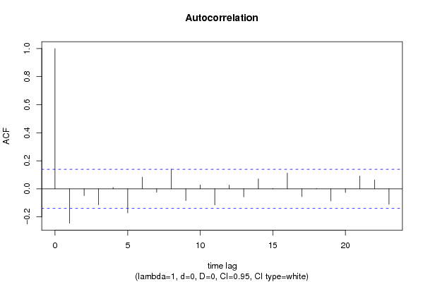
Title produced by software

(Partial) Autocorrelation Function

Date of computation

Mon, 22 Nov 2010 14:37:57 +0000

Cite this page as follows

Statistical Computations at FreeStatistics.org, Office for Research Development and Education, URL https://freestatistics.org/blog/index.php?v=date/2010/Nov/22/t1290436555euic2d7s42sd13r.htm/, Retrieved Sat, 04 May 2024 00:07:06 +0000

Statistical Computations at FreeStatistics.org, Office for Research Development and Education, URL https://freestatistics.org/blog/index.php?pk=98540, Retrieved Sat, 04 May 2024 00:07:06 +0000

QR Codes:

Paste this QR Code to cite your computation.

Original text written by user:

IsPrivate?

No (this computation is public)

User-defined keywords

Estimated Impact

107

Family? (F = Feedback message, R = changed R code, M = changed R Module, P = changed Parameters, D = changed Data)

-       [(Partial) Autocorrelation Function] [] [2010-11-22 14:37:57] [9b9a58c480cb5dafe4bfceb51e1cfd12] [Current]

Feedback Forum

Post a new message

Dataseries X:

Download CSV

Histogram

Boxplots

-1.8207657603853E-14
-0.018785294593818
-1.3322676295502E-15
-1.3322676295502E-15
-1.3322676295502E-15
-1.3322676295502E-15
-1.3322676295502E-15
-1.3322676295502E-15
-1.3322676295502E-15
-1.3322676295502E-15
-1.3322676295502E-15
-1.3322676295502E-15
-1.3322676295502E-15
0.018785294593799
-1.8207657603853E-14
-1.8207657603853E-14
-0.018785294593818
-1.3322676295502E-15
-1.3322676295502E-15
-1.3322676295502E-15
-1.3322676295502E-15
-1.3322676295502E-15
-1.3322676295502E-15
-1.3322676295502E-15
0.018785294593799
-0.018785294593818
-1.3322676295502E-15
0.018785294593799
-0.018785294593818
0.018785294593799
-1.8207657603853E-14
-1.8207657603853E-14
-0.018785294593818
-1.3322676295502E-15
0.018785294593799
-1.8207657603853E-14
-1.8207657603853E-14
-1.8207657603853E-14
-1.8207657603853E-14
-1.8207657603853E-14
-1.8207657603853E-14
-1.8207657603853E-14
-1.8207657603853E-14
-1.8207657603853E-14
-1.8207657603853E-14
-1.8207657603853E-14
-0.018785294593818
-1.3322676295502E-15
-1.3322676295502E-15
-1.3322676295502E-15
0.018785294593799
-1.8207657603853E-14
-1.8207657603853E-14
-1.8207657603853E-14
-1.8207657603853E-14
-0.018785294593818
0.018785294593799
-0.018785294593818
-1.3322676295502E-15
-1.3322676295502E-15
0.018785294593799
-0.018785294593818
-1.3322676295502E-15
-1.3322676295502E-15
-1.3322676295502E-15
0.018785294593799
-1.8207657603853E-14
-1.8207657603853E-14
-1.8207657603853E-14
-0.018785294593818
-1.3322676295502E-15
0.018785294593799
-1.8207657603853E-14
-1.8207657603853E-14
-1.8207657603853E-14
-1.8207657603853E-14
-0.018785294593818
0.018785294593799
-1.8207657603853E-14
-0.018785294593818
-1.3322676295502E-15
0.018785294593799
-1.8207657603853E-14
-1.8207657603853E-14
-1.8207657603853E-14
-1.8207657603853E-14
-1.8207657603853E-14
-1.8207657603853E-14
-1.8207657603853E-14
-1.8207657603853E-14
-1.8207657603853E-14
-0.018785294593818
-1.3322676295502E-15
-1.3322676295502E-15
-1.3322676295502E-15
-1.3322676295502E-15
0.018785294593799
-1.8207657603853E-14
-0.018785294593818
-1.3322676295502E-15
-1.3322676295502E-15
-1.3322676295502E-15
-1.3322676295502E-15
-1.3322676295502E-15
0.018785294593799
-1.8207657603853E-14
-0.018785294593818
-1.3322676295502E-15
-1.3322676295502E-15
-1.3322676295502E-15
-1.3322676295502E-15
-1.3322676295502E-15
0.018785294593799
-1.8207657603853E-14
-0.018785294593818
-1.3322676295502E-15
-1.3322676295502E-15
-1.3322676295502E-15
-1.3322676295502E-15
-1.3322676295502E-15
-1.3322676295502E-15
0.018785294593799
-1.8207657603853E-14
-1.8207657603853E-14
-1.8207657603853E-14
-1.8207657603853E-14
-1.8207657603853E-14
-0.018785294593818
-1.3322676295502E-15
0.018785294593799
-1.8207657603853E-14
-1.8207657603853E-14
-1.8207657603853E-14
-1.8207657603853E-14
-1.8207657603853E-14
-1.8207657603853E-14
-1.8207657603853E-14
0.014703375160182
-4.4853010194856E-14
-4.4853010194856E-14
-4.4853010194856E-14
-4.4853010194856E-14
-4.4853010194856E-14
-4.4853010194856E-14
-4.4853010194856E-14
-4.4853010194856E-14
-4.4853010194856E-14
-0.026546875584045
4.0856207306206E-14
4.0856207306206E-14
4.0856207306206E-14
0.026546875584041
-4.4853010194856E-14
-4.4853010194856E-14
-4.4853010194856E-14
-0.026546875584045
4.0856207306206E-14
4.0856207306206E-14
0.026546875584041
-4.4853010194856E-14
-0.00037432154654482
0.025869883192831
5.3290705182008E-15
5.3290705182008E-15
5.3290705182008E-15
5.3290705182008E-15
5.3290705182008E-15
5.3290705182008E-15
5.3290705182008E-15
5.3290705182008E-15
-0.025869883192795
3.0642155479654E-14
3.0642155479654E-14
3.0642155479654E-14
3.0642155479654E-14
0.025869883192831
-0.025869883192795
0.025869883192831
5.3290705182008E-15
5.3290705182008E-15
5.3290705182008E-15
5.3290705182008E-15
5.3290705182008E-15
5.3290705182008E-15
-0.025869883192795
3.0642155479654E-14
3.0642155479654E-14
0.025869883192831
5.3290705182008E-15
5.3290705182008E-15
-0.025869883192795
3.0642155479654E-14
3.0642155479654E-14
0.025869883192831
-0.025869883192795
0.025869883192831
5.3290705182008E-15
5.3290705182008E-15
-0.025869883192795
0.025869883192831

Summary of computational transaction
Raw Input	view raw input (R code)
Raw Output	view raw output of R engine
Computing time	2 seconds
R Server	'RServer@AstonUniversity' @ vre.aston.ac.uk

\begin{tabular}{lllllllll}
\hline
Summary of computational transaction \tabularnewline
Raw Input & view raw input (R code)  \tabularnewline
Raw Output & view raw output of R engine  \tabularnewline
Computing time & 2 seconds \tabularnewline
R Server & 'RServer@AstonUniversity' @ vre.aston.ac.uk \tabularnewline
\hline
\end{tabular}
%Source: https://freestatistics.org/blog/index.php?pk=98540&T=0

[TABLE]
[ROW][C]Summary of computational transaction[/C][/ROW]
[ROW][C]Raw Input[/C][C]view raw input (R code) [/C][/ROW]
[ROW][C]Raw Output[/C][C]view raw output of R engine [/C][/ROW]
[ROW][C]Computing time[/C][C]2 seconds[/C][/ROW]
[ROW][C]R Server[/C][C]'RServer@AstonUniversity' @ vre.aston.ac.uk[/C][/ROW]
[/TABLE]
Source: https://freestatistics.org/blog/index.php?pk=98540&T=0

Globally Unique Identifier (entire table): ba.freestatistics.org/blog/index.php?pk=98540&T=0

As an alternative you can also use a QR Code:

The GUIDs for individual cells are displayed in the table below:

Summary of computational transaction
Raw Input	view raw input (R code)
Raw Output	view raw output of R engine
Computing time	2 seconds
R Server	'RServer@AstonUniversity' @ vre.aston.ac.uk

Autocorrelation Function
Time lag k	ACF(k)	T-STAT	P-value
1	-0.245687	-3.4745	0.000314
2	-0.048622	-0.6876	0.246246
3	-0.114094	-1.6135	0.054103
4	0.009836	0.1391	0.444752
5	-0.172197	-2.4352	0.00788
6	0.083376	1.1791	0.119877
7	-0.025465	-0.3601	0.359564
8	0.140549	1.9877	0.024107
9	-0.083799	-1.1851	0.118693
10	0.027413	0.3877	0.349336
11	-0.114846	-1.6242	0.052958
12	0.02695	0.3811	0.351757
13	-0.057839	-0.818	0.207174
14	0.070445	0.9962	0.160169
15	0.003262	0.0461	0.481626
16	0.112719	1.5941	0.056248
17	-0.056614	-0.8006	0.212142
18	0.002803	0.0396	0.484211
19	-0.086695	-1.2261	0.11081
20	-0.026413	-0.3735	0.354571
21	0.091023	1.2873	0.099746
22	0.062825	0.8885	0.187674
23	-0.110953	-1.5691	0.059102

\begin{tabular}{lllllllll}
\hline
Autocorrelation Function \tabularnewline
Time lag k & ACF(k) & T-STAT & P-value \tabularnewline
1 & -0.245687 & -3.4745 & 0.000314 \tabularnewline
2 & -0.048622 & -0.6876 & 0.246246 \tabularnewline
3 & -0.114094 & -1.6135 & 0.054103 \tabularnewline
4 & 0.009836 & 0.1391 & 0.444752 \tabularnewline
5 & -0.172197 & -2.4352 & 0.00788 \tabularnewline
6 & 0.083376 & 1.1791 & 0.119877 \tabularnewline
7 & -0.025465 & -0.3601 & 0.359564 \tabularnewline
8 & 0.140549 & 1.9877 & 0.024107 \tabularnewline
9 & -0.083799 & -1.1851 & 0.118693 \tabularnewline
10 & 0.027413 & 0.3877 & 0.349336 \tabularnewline
11 & -0.114846 & -1.6242 & 0.052958 \tabularnewline
12 & 0.02695 & 0.3811 & 0.351757 \tabularnewline
13 & -0.057839 & -0.818 & 0.207174 \tabularnewline
14 & 0.070445 & 0.9962 & 0.160169 \tabularnewline
15 & 0.003262 & 0.0461 & 0.481626 \tabularnewline
16 & 0.112719 & 1.5941 & 0.056248 \tabularnewline
17 & -0.056614 & -0.8006 & 0.212142 \tabularnewline
18 & 0.002803 & 0.0396 & 0.484211 \tabularnewline
19 & -0.086695 & -1.2261 & 0.11081 \tabularnewline
20 & -0.026413 & -0.3735 & 0.354571 \tabularnewline
21 & 0.091023 & 1.2873 & 0.099746 \tabularnewline
22 & 0.062825 & 0.8885 & 0.187674 \tabularnewline
23 & -0.110953 & -1.5691 & 0.059102 \tabularnewline
\hline
\end{tabular}
%Source: https://freestatistics.org/blog/index.php?pk=98540&T=1

[TABLE]
[ROW][C]Autocorrelation Function[/C][/ROW]
[ROW][C]Time lag k[/C][C]ACF(k)[/C][C]T-STAT[/C][C]P-value[/C][/ROW]
[ROW][C]1[/C][C]-0.245687[/C][C]-3.4745[/C][C]0.000314[/C][/ROW]
[ROW][C]2[/C][C]-0.048622[/C][C]-0.6876[/C][C]0.246246[/C][/ROW]
[ROW][C]3[/C][C]-0.114094[/C][C]-1.6135[/C][C]0.054103[/C][/ROW]
[ROW][C]4[/C][C]0.009836[/C][C]0.1391[/C][C]0.444752[/C][/ROW]
[ROW][C]5[/C][C]-0.172197[/C][C]-2.4352[/C][C]0.00788[/C][/ROW]
[ROW][C]6[/C][C]0.083376[/C][C]1.1791[/C][C]0.119877[/C][/ROW]
[ROW][C]7[/C][C]-0.025465[/C][C]-0.3601[/C][C]0.359564[/C][/ROW]
[ROW][C]8[/C][C]0.140549[/C][C]1.9877[/C][C]0.024107[/C][/ROW]
[ROW][C]9[/C][C]-0.083799[/C][C]-1.1851[/C][C]0.118693[/C][/ROW]
[ROW][C]10[/C][C]0.027413[/C][C]0.3877[/C][C]0.349336[/C][/ROW]
[ROW][C]11[/C][C]-0.114846[/C][C]-1.6242[/C][C]0.052958[/C][/ROW]
[ROW][C]12[/C][C]0.02695[/C][C]0.3811[/C][C]0.351757[/C][/ROW]
[ROW][C]13[/C][C]-0.057839[/C][C]-0.818[/C][C]0.207174[/C][/ROW]
[ROW][C]14[/C][C]0.070445[/C][C]0.9962[/C][C]0.160169[/C][/ROW]
[ROW][C]15[/C][C]0.003262[/C][C]0.0461[/C][C]0.481626[/C][/ROW]
[ROW][C]16[/C][C]0.112719[/C][C]1.5941[/C][C]0.056248[/C][/ROW]
[ROW][C]17[/C][C]-0.056614[/C][C]-0.8006[/C][C]0.212142[/C][/ROW]
[ROW][C]18[/C][C]0.002803[/C][C]0.0396[/C][C]0.484211[/C][/ROW]
[ROW][C]19[/C][C]-0.086695[/C][C]-1.2261[/C][C]0.11081[/C][/ROW]
[ROW][C]20[/C][C]-0.026413[/C][C]-0.3735[/C][C]0.354571[/C][/ROW]
[ROW][C]21[/C][C]0.091023[/C][C]1.2873[/C][C]0.099746[/C][/ROW]
[ROW][C]22[/C][C]0.062825[/C][C]0.8885[/C][C]0.187674[/C][/ROW]
[ROW][C]23[/C][C]-0.110953[/C][C]-1.5691[/C][C]0.059102[/C][/ROW]
[/TABLE]
Source: https://freestatistics.org/blog/index.php?pk=98540&T=1

Globally Unique Identifier (entire table): ba.freestatistics.org/blog/index.php?pk=98540&T=1

As an alternative you can also use a QR Code:

The GUIDs for individual cells are displayed in the table below:

Autocorrelation Function
Time lag k	ACF(k)	T-STAT	P-value
1	-0.245687	-3.4745	0.000314
2	-0.048622	-0.6876	0.246246
3	-0.114094	-1.6135	0.054103
4	0.009836	0.1391	0.444752
5	-0.172197	-2.4352	0.00788
6	0.083376	1.1791	0.119877
7	-0.025465	-0.3601	0.359564
8	0.140549	1.9877	0.024107
9	-0.083799	-1.1851	0.118693
10	0.027413	0.3877	0.349336
11	-0.114846	-1.6242	0.052958
12	0.02695	0.3811	0.351757
13	-0.057839	-0.818	0.207174
14	0.070445	0.9962	0.160169
15	0.003262	0.0461	0.481626
16	0.112719	1.5941	0.056248
17	-0.056614	-0.8006	0.212142
18	0.002803	0.0396	0.484211
19	-0.086695	-1.2261	0.11081
20	-0.026413	-0.3735	0.354571
21	0.091023	1.2873	0.099746
22	0.062825	0.8885	0.187674
23	-0.110953	-1.5691	0.059102

Partial Autocorrelation Function
Time lag k	PACF(k)	T-STAT	P-value
1	-0.245687	-3.4745	0.000314
2	-0.115985	-1.6403	0.05126
3	-0.1682	-2.3787	0.009157
4	-0.080906	-1.1442	0.126956
5	-0.24403	-3.4511	0.000341
6	-0.077319	-1.0935	0.137753
7	-0.103147	-1.4587	0.073105
8	0.05364	0.7586	0.224496
9	-0.063018	-0.8912	0.186944
10	-0.03479	-0.492	0.311628
11	-0.121504	-1.7183	0.043642
12	-0.074534	-1.0541	0.146561
13	-0.094787	-1.3405	0.090803
14	-0.053054	-0.7503	0.226979
15	-0.038357	-0.5425	0.294054
16	0.042707	0.604	0.273273
17	-0.004447	-0.0629	0.474958
18	-0.011015	-0.1558	0.438184
19	-0.05461	-0.7723	0.220426
20	-0.093946	-1.3286	0.092747
21	0.076308	1.0792	0.140907
22	0.062101	0.8782	0.190434
23	-0.085356	-1.2071	0.114406

\begin{tabular}{lllllllll}
\hline
Partial Autocorrelation Function \tabularnewline
Time lag k & PACF(k) & T-STAT & P-value \tabularnewline
1 & -0.245687 & -3.4745 & 0.000314 \tabularnewline
2 & -0.115985 & -1.6403 & 0.05126 \tabularnewline
3 & -0.1682 & -2.3787 & 0.009157 \tabularnewline
4 & -0.080906 & -1.1442 & 0.126956 \tabularnewline
5 & -0.24403 & -3.4511 & 0.000341 \tabularnewline
6 & -0.077319 & -1.0935 & 0.137753 \tabularnewline
7 & -0.103147 & -1.4587 & 0.073105 \tabularnewline
8 & 0.05364 & 0.7586 & 0.224496 \tabularnewline
9 & -0.063018 & -0.8912 & 0.186944 \tabularnewline
10 & -0.03479 & -0.492 & 0.311628 \tabularnewline
11 & -0.121504 & -1.7183 & 0.043642 \tabularnewline
12 & -0.074534 & -1.0541 & 0.146561 \tabularnewline
13 & -0.094787 & -1.3405 & 0.090803 \tabularnewline
14 & -0.053054 & -0.7503 & 0.226979 \tabularnewline
15 & -0.038357 & -0.5425 & 0.294054 \tabularnewline
16 & 0.042707 & 0.604 & 0.273273 \tabularnewline
17 & -0.004447 & -0.0629 & 0.474958 \tabularnewline
18 & -0.011015 & -0.1558 & 0.438184 \tabularnewline
19 & -0.05461 & -0.7723 & 0.220426 \tabularnewline
20 & -0.093946 & -1.3286 & 0.092747 \tabularnewline
21 & 0.076308 & 1.0792 & 0.140907 \tabularnewline
22 & 0.062101 & 0.8782 & 0.190434 \tabularnewline
23 & -0.085356 & -1.2071 & 0.114406 \tabularnewline
\hline
\end{tabular}
%Source: https://freestatistics.org/blog/index.php?pk=98540&T=2

[TABLE]
[ROW][C]Partial Autocorrelation Function[/C][/ROW]
[ROW][C]Time lag k[/C][C]PACF(k)[/C][C]T-STAT[/C][C]P-value[/C][/ROW]
[ROW][C]1[/C][C]-0.245687[/C][C]-3.4745[/C][C]0.000314[/C][/ROW]
[ROW][C]2[/C][C]-0.115985[/C][C]-1.6403[/C][C]0.05126[/C][/ROW]
[ROW][C]3[/C][C]-0.1682[/C][C]-2.3787[/C][C]0.009157[/C][/ROW]
[ROW][C]4[/C][C]-0.080906[/C][C]-1.1442[/C][C]0.126956[/C][/ROW]
[ROW][C]5[/C][C]-0.24403[/C][C]-3.4511[/C][C]0.000341[/C][/ROW]
[ROW][C]6[/C][C]-0.077319[/C][C]-1.0935[/C][C]0.137753[/C][/ROW]
[ROW][C]7[/C][C]-0.103147[/C][C]-1.4587[/C][C]0.073105[/C][/ROW]
[ROW][C]8[/C][C]0.05364[/C][C]0.7586[/C][C]0.224496[/C][/ROW]
[ROW][C]9[/C][C]-0.063018[/C][C]-0.8912[/C][C]0.186944[/C][/ROW]
[ROW][C]10[/C][C]-0.03479[/C][C]-0.492[/C][C]0.311628[/C][/ROW]
[ROW][C]11[/C][C]-0.121504[/C][C]-1.7183[/C][C]0.043642[/C][/ROW]
[ROW][C]12[/C][C]-0.074534[/C][C]-1.0541[/C][C]0.146561[/C][/ROW]
[ROW][C]13[/C][C]-0.094787[/C][C]-1.3405[/C][C]0.090803[/C][/ROW]
[ROW][C]14[/C][C]-0.053054[/C][C]-0.7503[/C][C]0.226979[/C][/ROW]
[ROW][C]15[/C][C]-0.038357[/C][C]-0.5425[/C][C]0.294054[/C][/ROW]
[ROW][C]16[/C][C]0.042707[/C][C]0.604[/C][C]0.273273[/C][/ROW]
[ROW][C]17[/C][C]-0.004447[/C][C]-0.0629[/C][C]0.474958[/C][/ROW]
[ROW][C]18[/C][C]-0.011015[/C][C]-0.1558[/C][C]0.438184[/C][/ROW]
[ROW][C]19[/C][C]-0.05461[/C][C]-0.7723[/C][C]0.220426[/C][/ROW]
[ROW][C]20[/C][C]-0.093946[/C][C]-1.3286[/C][C]0.092747[/C][/ROW]
[ROW][C]21[/C][C]0.076308[/C][C]1.0792[/C][C]0.140907[/C][/ROW]
[ROW][C]22[/C][C]0.062101[/C][C]0.8782[/C][C]0.190434[/C][/ROW]
[ROW][C]23[/C][C]-0.085356[/C][C]-1.2071[/C][C]0.114406[/C][/ROW]
[/TABLE]
Source: https://freestatistics.org/blog/index.php?pk=98540&T=2

Globally Unique Identifier (entire table): ba.freestatistics.org/blog/index.php?pk=98540&T=2

As an alternative you can also use a QR Code:

The GUIDs for individual cells are displayed in the table below:

Partial Autocorrelation Function
Time lag k	PACF(k)	T-STAT	P-value
1	-0.245687	-3.4745	0.000314
2	-0.115985	-1.6403	0.05126
3	-0.1682	-2.3787	0.009157
4	-0.080906	-1.1442	0.126956
5	-0.24403	-3.4511	0.000341
6	-0.077319	-1.0935	0.137753
7	-0.103147	-1.4587	0.073105
8	0.05364	0.7586	0.224496
9	-0.063018	-0.8912	0.186944
10	-0.03479	-0.492	0.311628
11	-0.121504	-1.7183	0.043642
12	-0.074534	-1.0541	0.146561
13	-0.094787	-1.3405	0.090803
14	-0.053054	-0.7503	0.226979
15	-0.038357	-0.5425	0.294054
16	0.042707	0.604	0.273273
17	-0.004447	-0.0629	0.474958
18	-0.011015	-0.1558	0.438184
19	-0.05461	-0.7723	0.220426
20	-0.093946	-1.3286	0.092747
21	0.076308	1.0792	0.140907
22	0.062101	0.8782	0.190434
23	-0.085356	-1.2071	0.114406

Figure 1

PNG link

Postscript link

PDF link

Figure 2

PNG link

Postscript link

PDF link

Parameters (Session):

par1 = Default ; par2 = 1 ; par3 = 0 ; par4 = 0 ; par5 = 12 ; par6 = White Noise ; par7 = 0.95 ;

Parameters (R input):

par1 = Default ; par2 = 1 ; par3 = 0 ; par4 = 0 ; par5 = 12 ; par6 = White Noise ; par7 = 0.95 ;

R code (references can be found in the software module):

if (par1 == 'Default') {
par1 = 10*log10(length(x))
} else {
par1 <- as.numeric(par1)
}
par2 <- as.numeric(par2)
par3 <- as.numeric(par3)
par4 <- as.numeric(par4)
par5 <- as.numeric(par5)
if (par6 == 'White Noise') par6 <- 'white' else par6 <- 'ma'
par7 <- as.numeric(par7)
if (par2 == 0) {
x <- log(x)
} else {
x <- (x ^ par2 - 1) / par2
}
if (par3 > 0) x <- diff(x,lag=1,difference=par3)
if (par4 > 0) x <- diff(x,lag=par5,difference=par4)
bitmap(file='pic1.png')
racf <- acf(x, par1, main='Autocorrelation', xlab='time lag', ylab='ACF', ci.type=par6, ci=par7, sub=paste('(lambda=',par2,', d=',par3,', D=',par4,', CI=', par7, ', CI type=',par6,')',sep=''))
dev.off()
bitmap(file='pic2.png')
rpacf <- pacf(x,par1,main='Partial Autocorrelation',xlab='lags',ylab='PACF')
dev.off()
(myacf <- c(racf$acf))
(mypacf <- c(rpacf$acf))
lengthx <- length(x)
sqrtn <- sqrt(lengthx)
load(file='createtable')
a<-table.start()
a<-table.row.start(a)
a<-table.element(a,'Autocorrelation Function',4,TRUE)
a<-table.row.end(a)
a<-table.row.start(a)
a<-table.element(a,'Time lag k',header=TRUE)
a<-table.element(a,hyperlink('basics.htm','ACF(k)','click here for more information about the Autocorrelation Function'),header=TRUE)
a<-table.element(a,'T-STAT',header=TRUE)
a<-table.element(a,'P-value',header=TRUE)
a<-table.row.end(a)
for (i in 2:(par1+1)) {
a<-table.row.start(a)
a<-table.element(a,i-1,header=TRUE)
a<-table.element(a,round(myacf[i],6))
mytstat <- myacf[i]*sqrtn
a<-table.element(a,round(mytstat,4))
a<-table.element(a,round(1-pt(abs(mytstat),lengthx),6))
a<-table.row.end(a)
}
a<-table.end(a)
table.save(a,file='mytable.tab')
a<-table.start()
a<-table.row.start(a)
a<-table.element(a,'Partial Autocorrelation Function',4,TRUE)
a<-table.row.end(a)
a<-table.row.start(a)
a<-table.element(a,'Time lag k',header=TRUE)
a<-table.element(a,hyperlink('basics.htm','PACF(k)','click here for more information about the Partial Autocorrelation Function'),header=TRUE)
a<-table.element(a,'T-STAT',header=TRUE)
a<-table.element(a,'P-value',header=TRUE)
a<-table.row.end(a)
for (i in 1:par1) {
a<-table.row.start(a)
a<-table.element(a,i,header=TRUE)
a<-table.element(a,round(mypacf[i],6))
mytstat <- mypacf[i]*sqrtn
a<-table.element(a,round(mytstat,4))
a<-table.element(a,round(1-pt(abs(mytstat),lengthx),6))
a<-table.row.end(a)
}
a<-table.end(a)
table.save(a,file='mytable1.tab')

Free Statistics

Description of Statistical Computation

Tree of Dependent Computations

Dataset

Tables (Output of Computation)

Figures (Output of Computation)

Input Parameters & R Code