Repository of Reproducible Computations

Free Statistics

of Irreproducible Research!

Author's title

Author

*Unverified author*

R Software Module

rwasp_autocorrelation.wasp

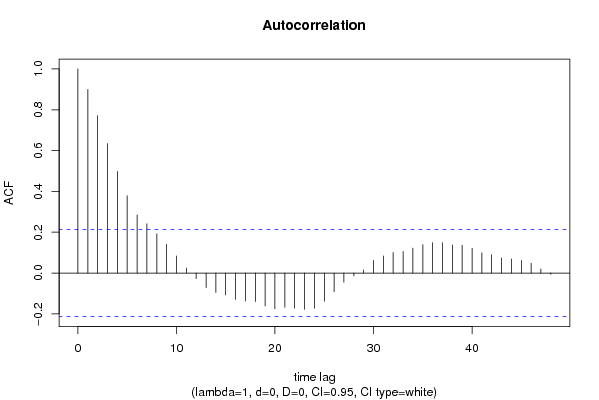
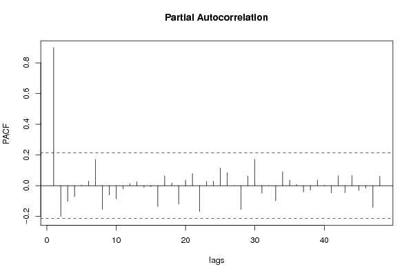
Title produced by software

(Partial) Autocorrelation Function

Date of computation

Sat, 20 Nov 2010 16:49:25 +0000

Cite this page as follows

Statistical Computations at FreeStatistics.org, Office for Research Development and Education, URL https://freestatistics.org/blog/index.php?v=date/2010/Nov/20/t1290271925ob8rgo5ediwaox5.htm/, Retrieved Sat, 27 Apr 2024 07:11:10 +0000

Statistical Computations at FreeStatistics.org, Office for Research Development and Education, URL https://freestatistics.org/blog/index.php?pk=98269, Retrieved Sat, 27 Apr 2024 07:11:10 +0000

QR Codes:

Paste this QR Code to cite your computation.

Original text written by user:

IsPrivate?

No (this computation is public)

User-defined keywords

KDGP2W12 - Kristina Henderickx

Estimated Impact

107

Family? (F = Feedback message, R = changed R code, M = changed R Module, P = changed Parameters, D = changed Data)

-       [(Partial) Autocorrelation Function] [Aurocorrelation c...] [2010-11-20 16:49:25] [85d6e4146de3ee96ae2a9c7dd566a647] [Current]

Feedback Forum

Post a new message

Dataseries X:

Download CSV

Histogram

Boxplots

0,65
0,65
0,65
0,65
0,65
0,65
0,66
0,66
0,66
0,65
0,65
0,65
0,65
0,65
0,65
0,65
0,66
0,67
0,66
0,67
0,66
0,66
0,66
0,66
0,71
0,74
0,75
0,75
0,75
0,75
0,7
0,69
0,69
0,68
0,68
0,68
0,67
0,66
0,66
0,67
0,67
0,67
0,67
0,68
0,68
0,67
0,67
0,67
0,67
0,67
0,69
0,69
0,69
0,69
0,69
0,69
0,7
0,69
0,68
0,7
0,7
0,71
0,69
0,7
0,7
0,71
0,71
0,71
0,71
0,7
0,7
0,71
0,71
0,71
0,71
0,7
0,69
0,7
0,7
0,7
0,71
0,7
0,7
0,69

Summary of computational transaction
Raw Input	view raw input (R code)
Raw Output	view raw output of R engine
Computing time	1 seconds
R Server	'George Udny Yule' @ 72.249.76.132

\begin{tabular}{lllllllll}
\hline
Summary of computational transaction \tabularnewline
Raw Input & view raw input (R code)  \tabularnewline
Raw Output & view raw output of R engine  \tabularnewline
Computing time & 1 seconds \tabularnewline
R Server & 'George Udny Yule' @ 72.249.76.132 \tabularnewline
\hline
\end{tabular}
%Source: https://freestatistics.org/blog/index.php?pk=98269&T=0

[TABLE]
[ROW][C]Summary of computational transaction[/C][/ROW]
[ROW][C]Raw Input[/C][C]view raw input (R code) [/C][/ROW]
[ROW][C]Raw Output[/C][C]view raw output of R engine [/C][/ROW]
[ROW][C]Computing time[/C][C]1 seconds[/C][/ROW]
[ROW][C]R Server[/C][C]'George Udny Yule' @ 72.249.76.132[/C][/ROW]
[/TABLE]
Source: https://freestatistics.org/blog/index.php?pk=98269&T=0

Globally Unique Identifier (entire table): ba.freestatistics.org/blog/index.php?pk=98269&T=0

As an alternative you can also use a QR Code:

The GUIDs for individual cells are displayed in the table below:

Summary of computational transaction
Raw Input	view raw input (R code)
Raw Output	view raw output of R engine
Computing time	1 seconds
R Server	'George Udny Yule' @ 72.249.76.132

Autocorrelation Function
Time lag k	ACF(k)	T-STAT	P-value
1	0.899732	8.2462	0
2	0.771528	7.0712	0
3	0.634367	5.8141	0
4	0.49793	4.5636	9e-06
5	0.378683	3.4707	0.000411
6	0.284514	2.6076	0.005394
7	0.241228	2.2109	0.01488
8	0.191843	1.7583	0.041172
9	0.141392	1.2959	0.099284
10	0.083775	0.7678	0.222376
11	0.024367	0.2233	0.411911
12	-0.027876	-0.2555	0.399487
13	-0.071161	-0.6522	0.258025
14	-0.095468	-0.875	0.192041
15	-0.107234	-0.9828	0.16426
16	-0.129024	-1.1825	0.120167
17	-0.137549	-1.2607	0.105461
18	-0.139975	-1.2829	0.101529
19	-0.16104	-1.476	0.071848
20	-0.174939	-1.6033	0.056306
21	-0.168067	-1.5404	0.063616
22	-0.172668	-1.5825	0.058643
23	-0.177611	-1.6278	0.053653
24	-0.17253	-1.5813	0.058788
25	-0.138745	-1.2716	0.103508
26	-0.091696	-0.8404	0.201533
27	-0.044988	-0.4123	0.340577
28	-0.013677	-0.1254	0.450273
29	0.015118	0.1386	0.445066
30	0.061826	0.5666	0.286233
31	0.083413	0.7645	0.223359
32	0.100691	0.9229	0.179364
33	0.105431	0.9663	0.168337
34	0.121984	1.118	0.133376
35	0.138879	1.2729	0.103291
36	0.148609	1.362	0.088416
37	0.148657	1.3625	0.088347
38	0.137231	1.2577	0.105985
39	0.136554	1.2515	0.107106
40	0.121205	1.1109	0.1349
41	0.09869	0.9045	0.184157
42	0.089781	0.8229	0.20646
43	0.073706	0.6755	0.250597
44	0.069105	0.6334	0.26411
45	0.060921	0.5584	0.289045
46	0.047704	0.4372	0.331538
47	0.020157	0.1847	0.426939
48	-0.006666	-0.0611	0.475715

\begin{tabular}{lllllllll}
\hline
Autocorrelation Function \tabularnewline
Time lag k & ACF(k) & T-STAT & P-value \tabularnewline
1 & 0.899732 & 8.2462 & 0 \tabularnewline
2 & 0.771528 & 7.0712 & 0 \tabularnewline
3 & 0.634367 & 5.8141 & 0 \tabularnewline
4 & 0.49793 & 4.5636 & 9e-06 \tabularnewline
5 & 0.378683 & 3.4707 & 0.000411 \tabularnewline
6 & 0.284514 & 2.6076 & 0.005394 \tabularnewline
7 & 0.241228 & 2.2109 & 0.01488 \tabularnewline
8 & 0.191843 & 1.7583 & 0.041172 \tabularnewline
9 & 0.141392 & 1.2959 & 0.099284 \tabularnewline
10 & 0.083775 & 0.7678 & 0.222376 \tabularnewline
11 & 0.024367 & 0.2233 & 0.411911 \tabularnewline
12 & -0.027876 & -0.2555 & 0.399487 \tabularnewline
13 & -0.071161 & -0.6522 & 0.258025 \tabularnewline
14 & -0.095468 & -0.875 & 0.192041 \tabularnewline
15 & -0.107234 & -0.9828 & 0.16426 \tabularnewline
16 & -0.129024 & -1.1825 & 0.120167 \tabularnewline
17 & -0.137549 & -1.2607 & 0.105461 \tabularnewline
18 & -0.139975 & -1.2829 & 0.101529 \tabularnewline
19 & -0.16104 & -1.476 & 0.071848 \tabularnewline
20 & -0.174939 & -1.6033 & 0.056306 \tabularnewline
21 & -0.168067 & -1.5404 & 0.063616 \tabularnewline
22 & -0.172668 & -1.5825 & 0.058643 \tabularnewline
23 & -0.177611 & -1.6278 & 0.053653 \tabularnewline
24 & -0.17253 & -1.5813 & 0.058788 \tabularnewline
25 & -0.138745 & -1.2716 & 0.103508 \tabularnewline
26 & -0.091696 & -0.8404 & 0.201533 \tabularnewline
27 & -0.044988 & -0.4123 & 0.340577 \tabularnewline
28 & -0.013677 & -0.1254 & 0.450273 \tabularnewline
29 & 0.015118 & 0.1386 & 0.445066 \tabularnewline
30 & 0.061826 & 0.5666 & 0.286233 \tabularnewline
31 & 0.083413 & 0.7645 & 0.223359 \tabularnewline
32 & 0.100691 & 0.9229 & 0.179364 \tabularnewline
33 & 0.105431 & 0.9663 & 0.168337 \tabularnewline
34 & 0.121984 & 1.118 & 0.133376 \tabularnewline
35 & 0.138879 & 1.2729 & 0.103291 \tabularnewline
36 & 0.148609 & 1.362 & 0.088416 \tabularnewline
37 & 0.148657 & 1.3625 & 0.088347 \tabularnewline
38 & 0.137231 & 1.2577 & 0.105985 \tabularnewline
39 & 0.136554 & 1.2515 & 0.107106 \tabularnewline
40 & 0.121205 & 1.1109 & 0.1349 \tabularnewline
41 & 0.09869 & 0.9045 & 0.184157 \tabularnewline
42 & 0.089781 & 0.8229 & 0.20646 \tabularnewline
43 & 0.073706 & 0.6755 & 0.250597 \tabularnewline
44 & 0.069105 & 0.6334 & 0.26411 \tabularnewline
45 & 0.060921 & 0.5584 & 0.289045 \tabularnewline
46 & 0.047704 & 0.4372 & 0.331538 \tabularnewline
47 & 0.020157 & 0.1847 & 0.426939 \tabularnewline
48 & -0.006666 & -0.0611 & 0.475715 \tabularnewline
\hline
\end{tabular}
%Source: https://freestatistics.org/blog/index.php?pk=98269&T=1

[TABLE]
[ROW][C]Autocorrelation Function[/C][/ROW]
[ROW][C]Time lag k[/C][C]ACF(k)[/C][C]T-STAT[/C][C]P-value[/C][/ROW]
[ROW][C]1[/C][C]0.899732[/C][C]8.2462[/C][C]0[/C][/ROW]
[ROW][C]2[/C][C]0.771528[/C][C]7.0712[/C][C]0[/C][/ROW]
[ROW][C]3[/C][C]0.634367[/C][C]5.8141[/C][C]0[/C][/ROW]
[ROW][C]4[/C][C]0.49793[/C][C]4.5636[/C][C]9e-06[/C][/ROW]
[ROW][C]5[/C][C]0.378683[/C][C]3.4707[/C][C]0.000411[/C][/ROW]
[ROW][C]6[/C][C]0.284514[/C][C]2.6076[/C][C]0.005394[/C][/ROW]
[ROW][C]7[/C][C]0.241228[/C][C]2.2109[/C][C]0.01488[/C][/ROW]
[ROW][C]8[/C][C]0.191843[/C][C]1.7583[/C][C]0.041172[/C][/ROW]
[ROW][C]9[/C][C]0.141392[/C][C]1.2959[/C][C]0.099284[/C][/ROW]
[ROW][C]10[/C][C]0.083775[/C][C]0.7678[/C][C]0.222376[/C][/ROW]
[ROW][C]11[/C][C]0.024367[/C][C]0.2233[/C][C]0.411911[/C][/ROW]
[ROW][C]12[/C][C]-0.027876[/C][C]-0.2555[/C][C]0.399487[/C][/ROW]
[ROW][C]13[/C][C]-0.071161[/C][C]-0.6522[/C][C]0.258025[/C][/ROW]
[ROW][C]14[/C][C]-0.095468[/C][C]-0.875[/C][C]0.192041[/C][/ROW]
[ROW][C]15[/C][C]-0.107234[/C][C]-0.9828[/C][C]0.16426[/C][/ROW]
[ROW][C]16[/C][C]-0.129024[/C][C]-1.1825[/C][C]0.120167[/C][/ROW]
[ROW][C]17[/C][C]-0.137549[/C][C]-1.2607[/C][C]0.105461[/C][/ROW]
[ROW][C]18[/C][C]-0.139975[/C][C]-1.2829[/C][C]0.101529[/C][/ROW]
[ROW][C]19[/C][C]-0.16104[/C][C]-1.476[/C][C]0.071848[/C][/ROW]
[ROW][C]20[/C][C]-0.174939[/C][C]-1.6033[/C][C]0.056306[/C][/ROW]
[ROW][C]21[/C][C]-0.168067[/C][C]-1.5404[/C][C]0.063616[/C][/ROW]
[ROW][C]22[/C][C]-0.172668[/C][C]-1.5825[/C][C]0.058643[/C][/ROW]
[ROW][C]23[/C][C]-0.177611[/C][C]-1.6278[/C][C]0.053653[/C][/ROW]
[ROW][C]24[/C][C]-0.17253[/C][C]-1.5813[/C][C]0.058788[/C][/ROW]
[ROW][C]25[/C][C]-0.138745[/C][C]-1.2716[/C][C]0.103508[/C][/ROW]
[ROW][C]26[/C][C]-0.091696[/C][C]-0.8404[/C][C]0.201533[/C][/ROW]
[ROW][C]27[/C][C]-0.044988[/C][C]-0.4123[/C][C]0.340577[/C][/ROW]
[ROW][C]28[/C][C]-0.013677[/C][C]-0.1254[/C][C]0.450273[/C][/ROW]
[ROW][C]29[/C][C]0.015118[/C][C]0.1386[/C][C]0.445066[/C][/ROW]
[ROW][C]30[/C][C]0.061826[/C][C]0.5666[/C][C]0.286233[/C][/ROW]
[ROW][C]31[/C][C]0.083413[/C][C]0.7645[/C][C]0.223359[/C][/ROW]
[ROW][C]32[/C][C]0.100691[/C][C]0.9229[/C][C]0.179364[/C][/ROW]
[ROW][C]33[/C][C]0.105431[/C][C]0.9663[/C][C]0.168337[/C][/ROW]
[ROW][C]34[/C][C]0.121984[/C][C]1.118[/C][C]0.133376[/C][/ROW]
[ROW][C]35[/C][C]0.138879[/C][C]1.2729[/C][C]0.103291[/C][/ROW]
[ROW][C]36[/C][C]0.148609[/C][C]1.362[/C][C]0.088416[/C][/ROW]
[ROW][C]37[/C][C]0.148657[/C][C]1.3625[/C][C]0.088347[/C][/ROW]
[ROW][C]38[/C][C]0.137231[/C][C]1.2577[/C][C]0.105985[/C][/ROW]
[ROW][C]39[/C][C]0.136554[/C][C]1.2515[/C][C]0.107106[/C][/ROW]
[ROW][C]40[/C][C]0.121205[/C][C]1.1109[/C][C]0.1349[/C][/ROW]
[ROW][C]41[/C][C]0.09869[/C][C]0.9045[/C][C]0.184157[/C][/ROW]
[ROW][C]42[/C][C]0.089781[/C][C]0.8229[/C][C]0.20646[/C][/ROW]
[ROW][C]43[/C][C]0.073706[/C][C]0.6755[/C][C]0.250597[/C][/ROW]
[ROW][C]44[/C][C]0.069105[/C][C]0.6334[/C][C]0.26411[/C][/ROW]
[ROW][C]45[/C][C]0.060921[/C][C]0.5584[/C][C]0.289045[/C][/ROW]
[ROW][C]46[/C][C]0.047704[/C][C]0.4372[/C][C]0.331538[/C][/ROW]
[ROW][C]47[/C][C]0.020157[/C][C]0.1847[/C][C]0.426939[/C][/ROW]
[ROW][C]48[/C][C]-0.006666[/C][C]-0.0611[/C][C]0.475715[/C][/ROW]
[/TABLE]
Source: https://freestatistics.org/blog/index.php?pk=98269&T=1

Globally Unique Identifier (entire table): ba.freestatistics.org/blog/index.php?pk=98269&T=1

As an alternative you can also use a QR Code:

The GUIDs for individual cells are displayed in the table below:

Autocorrelation Function
Time lag k	ACF(k)	T-STAT	P-value
1	0.899732	8.2462	0
2	0.771528	7.0712	0
3	0.634367	5.8141	0
4	0.49793	4.5636	9e-06
5	0.378683	3.4707	0.000411
6	0.284514	2.6076	0.005394
7	0.241228	2.2109	0.01488
8	0.191843	1.7583	0.041172
9	0.141392	1.2959	0.099284
10	0.083775	0.7678	0.222376
11	0.024367	0.2233	0.411911
12	-0.027876	-0.2555	0.399487
13	-0.071161	-0.6522	0.258025
14	-0.095468	-0.875	0.192041
15	-0.107234	-0.9828	0.16426
16	-0.129024	-1.1825	0.120167
17	-0.137549	-1.2607	0.105461
18	-0.139975	-1.2829	0.101529
19	-0.16104	-1.476	0.071848
20	-0.174939	-1.6033	0.056306
21	-0.168067	-1.5404	0.063616
22	-0.172668	-1.5825	0.058643
23	-0.177611	-1.6278	0.053653
24	-0.17253	-1.5813	0.058788
25	-0.138745	-1.2716	0.103508
26	-0.091696	-0.8404	0.201533
27	-0.044988	-0.4123	0.340577
28	-0.013677	-0.1254	0.450273
29	0.015118	0.1386	0.445066
30	0.061826	0.5666	0.286233
31	0.083413	0.7645	0.223359
32	0.100691	0.9229	0.179364
33	0.105431	0.9663	0.168337
34	0.121984	1.118	0.133376
35	0.138879	1.2729	0.103291
36	0.148609	1.362	0.088416
37	0.148657	1.3625	0.088347
38	0.137231	1.2577	0.105985
39	0.136554	1.2515	0.107106
40	0.121205	1.1109	0.1349
41	0.09869	0.9045	0.184157
42	0.089781	0.8229	0.20646
43	0.073706	0.6755	0.250597
44	0.069105	0.6334	0.26411
45	0.060921	0.5584	0.289045
46	0.047704	0.4372	0.331538
47	0.020157	0.1847	0.426939
48	-0.006666	-0.0611	0.475715

Partial Autocorrelation Function
Time lag k	PACF(k)	T-STAT	P-value
1	0.899732	8.2462	0
2	-0.199442	-1.8279	0.035556
3	-0.102805	-0.9422	0.17439
4	-0.071177	-0.6523	0.257979
5	0.00298	0.0273	0.489137
6	0.029719	0.2724	0.392998
7	0.170387	1.5616	0.061068
8	-0.154406	-1.4152	0.080359
9	-0.060369	-0.5533	0.290767
10	-0.085632	-0.7848	0.217381
11	-0.021156	-0.1939	0.423362
12	0.012927	0.1185	0.452987
13	0.024763	0.227	0.410505
14	-0.011012	-0.1009	0.459926
15	-0.007104	-0.0651	0.47412
16	-0.136084	-1.2472	0.10789
17	0.063542	0.5824	0.280938
18	0.017431	0.1598	0.436728
19	-0.11931	-1.0935	0.138652
20	0.036833	0.3376	0.36826
21	0.078871	0.7229	0.235885
22	-0.168627	-1.5455	0.062994
23	0.027512	0.2522	0.400769
24	0.02882	0.2641	0.396161
25	0.11528	1.0566	0.146872
26	0.084332	0.7729	0.22087
27	-0.000608	-0.0056	0.497782
28	-0.156075	-1.4305	0.078148
29	0.06306	0.578	0.282422
30	0.170707	1.5646	0.060723
31	-0.049521	-0.4539	0.325549
32	0.00239	0.0219	0.491288
33	-0.09872	-0.9048	0.184084
34	0.090849	0.8326	0.203703
35	0.035688	0.3271	0.372208
36	0.007355	0.0674	0.473208
37	-0.040783	-0.3738	0.354755
38	-0.028358	-0.2599	0.397788
39	0.036493	0.3345	0.369432
40	0.002484	0.0228	0.490944
41	-0.047092	-0.4316	0.333568
42	0.063679	0.5836	0.280519
43	-0.045425	-0.4163	0.339116
44	0.065787	0.6029	0.274085
45	-0.031261	-0.2865	0.387595
46	-0.016048	-0.1471	0.441711
47	-0.142128	-1.3026	0.098132
48	0.061668	0.5652	0.286723

\begin{tabular}{lllllllll}
\hline
Partial Autocorrelation Function \tabularnewline
Time lag k & PACF(k) & T-STAT & P-value \tabularnewline
1 & 0.899732 & 8.2462 & 0 \tabularnewline
2 & -0.199442 & -1.8279 & 0.035556 \tabularnewline
3 & -0.102805 & -0.9422 & 0.17439 \tabularnewline
4 & -0.071177 & -0.6523 & 0.257979 \tabularnewline
5 & 0.00298 & 0.0273 & 0.489137 \tabularnewline
6 & 0.029719 & 0.2724 & 0.392998 \tabularnewline
7 & 0.170387 & 1.5616 & 0.061068 \tabularnewline
8 & -0.154406 & -1.4152 & 0.080359 \tabularnewline
9 & -0.060369 & -0.5533 & 0.290767 \tabularnewline
10 & -0.085632 & -0.7848 & 0.217381 \tabularnewline
11 & -0.021156 & -0.1939 & 0.423362 \tabularnewline
12 & 0.012927 & 0.1185 & 0.452987 \tabularnewline
13 & 0.024763 & 0.227 & 0.410505 \tabularnewline
14 & -0.011012 & -0.1009 & 0.459926 \tabularnewline
15 & -0.007104 & -0.0651 & 0.47412 \tabularnewline
16 & -0.136084 & -1.2472 & 0.10789 \tabularnewline
17 & 0.063542 & 0.5824 & 0.280938 \tabularnewline
18 & 0.017431 & 0.1598 & 0.436728 \tabularnewline
19 & -0.11931 & -1.0935 & 0.138652 \tabularnewline
20 & 0.036833 & 0.3376 & 0.36826 \tabularnewline
21 & 0.078871 & 0.7229 & 0.235885 \tabularnewline
22 & -0.168627 & -1.5455 & 0.062994 \tabularnewline
23 & 0.027512 & 0.2522 & 0.400769 \tabularnewline
24 & 0.02882 & 0.2641 & 0.396161 \tabularnewline
25 & 0.11528 & 1.0566 & 0.146872 \tabularnewline
26 & 0.084332 & 0.7729 & 0.22087 \tabularnewline
27 & -0.000608 & -0.0056 & 0.497782 \tabularnewline
28 & -0.156075 & -1.4305 & 0.078148 \tabularnewline
29 & 0.06306 & 0.578 & 0.282422 \tabularnewline
30 & 0.170707 & 1.5646 & 0.060723 \tabularnewline
31 & -0.049521 & -0.4539 & 0.325549 \tabularnewline
32 & 0.00239 & 0.0219 & 0.491288 \tabularnewline
33 & -0.09872 & -0.9048 & 0.184084 \tabularnewline
34 & 0.090849 & 0.8326 & 0.203703 \tabularnewline
35 & 0.035688 & 0.3271 & 0.372208 \tabularnewline
36 & 0.007355 & 0.0674 & 0.473208 \tabularnewline
37 & -0.040783 & -0.3738 & 0.354755 \tabularnewline
38 & -0.028358 & -0.2599 & 0.397788 \tabularnewline
39 & 0.036493 & 0.3345 & 0.369432 \tabularnewline
40 & 0.002484 & 0.0228 & 0.490944 \tabularnewline
41 & -0.047092 & -0.4316 & 0.333568 \tabularnewline
42 & 0.063679 & 0.5836 & 0.280519 \tabularnewline
43 & -0.045425 & -0.4163 & 0.339116 \tabularnewline
44 & 0.065787 & 0.6029 & 0.274085 \tabularnewline
45 & -0.031261 & -0.2865 & 0.387595 \tabularnewline
46 & -0.016048 & -0.1471 & 0.441711 \tabularnewline
47 & -0.142128 & -1.3026 & 0.098132 \tabularnewline
48 & 0.061668 & 0.5652 & 0.286723 \tabularnewline
\hline
\end{tabular}
%Source: https://freestatistics.org/blog/index.php?pk=98269&T=2

[TABLE]
[ROW][C]Partial Autocorrelation Function[/C][/ROW]
[ROW][C]Time lag k[/C][C]PACF(k)[/C][C]T-STAT[/C][C]P-value[/C][/ROW]
[ROW][C]1[/C][C]0.899732[/C][C]8.2462[/C][C]0[/C][/ROW]
[ROW][C]2[/C][C]-0.199442[/C][C]-1.8279[/C][C]0.035556[/C][/ROW]
[ROW][C]3[/C][C]-0.102805[/C][C]-0.9422[/C][C]0.17439[/C][/ROW]
[ROW][C]4[/C][C]-0.071177[/C][C]-0.6523[/C][C]0.257979[/C][/ROW]
[ROW][C]5[/C][C]0.00298[/C][C]0.0273[/C][C]0.489137[/C][/ROW]
[ROW][C]6[/C][C]0.029719[/C][C]0.2724[/C][C]0.392998[/C][/ROW]
[ROW][C]7[/C][C]0.170387[/C][C]1.5616[/C][C]0.061068[/C][/ROW]
[ROW][C]8[/C][C]-0.154406[/C][C]-1.4152[/C][C]0.080359[/C][/ROW]
[ROW][C]9[/C][C]-0.060369[/C][C]-0.5533[/C][C]0.290767[/C][/ROW]
[ROW][C]10[/C][C]-0.085632[/C][C]-0.7848[/C][C]0.217381[/C][/ROW]
[ROW][C]11[/C][C]-0.021156[/C][C]-0.1939[/C][C]0.423362[/C][/ROW]
[ROW][C]12[/C][C]0.012927[/C][C]0.1185[/C][C]0.452987[/C][/ROW]
[ROW][C]13[/C][C]0.024763[/C][C]0.227[/C][C]0.410505[/C][/ROW]
[ROW][C]14[/C][C]-0.011012[/C][C]-0.1009[/C][C]0.459926[/C][/ROW]
[ROW][C]15[/C][C]-0.007104[/C][C]-0.0651[/C][C]0.47412[/C][/ROW]
[ROW][C]16[/C][C]-0.136084[/C][C]-1.2472[/C][C]0.10789[/C][/ROW]
[ROW][C]17[/C][C]0.063542[/C][C]0.5824[/C][C]0.280938[/C][/ROW]
[ROW][C]18[/C][C]0.017431[/C][C]0.1598[/C][C]0.436728[/C][/ROW]
[ROW][C]19[/C][C]-0.11931[/C][C]-1.0935[/C][C]0.138652[/C][/ROW]
[ROW][C]20[/C][C]0.036833[/C][C]0.3376[/C][C]0.36826[/C][/ROW]
[ROW][C]21[/C][C]0.078871[/C][C]0.7229[/C][C]0.235885[/C][/ROW]
[ROW][C]22[/C][C]-0.168627[/C][C]-1.5455[/C][C]0.062994[/C][/ROW]
[ROW][C]23[/C][C]0.027512[/C][C]0.2522[/C][C]0.400769[/C][/ROW]
[ROW][C]24[/C][C]0.02882[/C][C]0.2641[/C][C]0.396161[/C][/ROW]
[ROW][C]25[/C][C]0.11528[/C][C]1.0566[/C][C]0.146872[/C][/ROW]
[ROW][C]26[/C][C]0.084332[/C][C]0.7729[/C][C]0.22087[/C][/ROW]
[ROW][C]27[/C][C]-0.000608[/C][C]-0.0056[/C][C]0.497782[/C][/ROW]
[ROW][C]28[/C][C]-0.156075[/C][C]-1.4305[/C][C]0.078148[/C][/ROW]
[ROW][C]29[/C][C]0.06306[/C][C]0.578[/C][C]0.282422[/C][/ROW]
[ROW][C]30[/C][C]0.170707[/C][C]1.5646[/C][C]0.060723[/C][/ROW]
[ROW][C]31[/C][C]-0.049521[/C][C]-0.4539[/C][C]0.325549[/C][/ROW]
[ROW][C]32[/C][C]0.00239[/C][C]0.0219[/C][C]0.491288[/C][/ROW]
[ROW][C]33[/C][C]-0.09872[/C][C]-0.9048[/C][C]0.184084[/C][/ROW]
[ROW][C]34[/C][C]0.090849[/C][C]0.8326[/C][C]0.203703[/C][/ROW]
[ROW][C]35[/C][C]0.035688[/C][C]0.3271[/C][C]0.372208[/C][/ROW]
[ROW][C]36[/C][C]0.007355[/C][C]0.0674[/C][C]0.473208[/C][/ROW]
[ROW][C]37[/C][C]-0.040783[/C][C]-0.3738[/C][C]0.354755[/C][/ROW]
[ROW][C]38[/C][C]-0.028358[/C][C]-0.2599[/C][C]0.397788[/C][/ROW]
[ROW][C]39[/C][C]0.036493[/C][C]0.3345[/C][C]0.369432[/C][/ROW]
[ROW][C]40[/C][C]0.002484[/C][C]0.0228[/C][C]0.490944[/C][/ROW]
[ROW][C]41[/C][C]-0.047092[/C][C]-0.4316[/C][C]0.333568[/C][/ROW]
[ROW][C]42[/C][C]0.063679[/C][C]0.5836[/C][C]0.280519[/C][/ROW]
[ROW][C]43[/C][C]-0.045425[/C][C]-0.4163[/C][C]0.339116[/C][/ROW]
[ROW][C]44[/C][C]0.065787[/C][C]0.6029[/C][C]0.274085[/C][/ROW]
[ROW][C]45[/C][C]-0.031261[/C][C]-0.2865[/C][C]0.387595[/C][/ROW]
[ROW][C]46[/C][C]-0.016048[/C][C]-0.1471[/C][C]0.441711[/C][/ROW]
[ROW][C]47[/C][C]-0.142128[/C][C]-1.3026[/C][C]0.098132[/C][/ROW]
[ROW][C]48[/C][C]0.061668[/C][C]0.5652[/C][C]0.286723[/C][/ROW]
[/TABLE]
Source: https://freestatistics.org/blog/index.php?pk=98269&T=2

Globally Unique Identifier (entire table): ba.freestatistics.org/blog/index.php?pk=98269&T=2

As an alternative you can also use a QR Code:

The GUIDs for individual cells are displayed in the table below:

Partial Autocorrelation Function
Time lag k	PACF(k)	T-STAT	P-value
1	0.899732	8.2462	0
2	-0.199442	-1.8279	0.035556
3	-0.102805	-0.9422	0.17439
4	-0.071177	-0.6523	0.257979
5	0.00298	0.0273	0.489137
6	0.029719	0.2724	0.392998
7	0.170387	1.5616	0.061068
8	-0.154406	-1.4152	0.080359
9	-0.060369	-0.5533	0.290767
10	-0.085632	-0.7848	0.217381
11	-0.021156	-0.1939	0.423362
12	0.012927	0.1185	0.452987
13	0.024763	0.227	0.410505
14	-0.011012	-0.1009	0.459926
15	-0.007104	-0.0651	0.47412
16	-0.136084	-1.2472	0.10789
17	0.063542	0.5824	0.280938
18	0.017431	0.1598	0.436728
19	-0.11931	-1.0935	0.138652
20	0.036833	0.3376	0.36826
21	0.078871	0.7229	0.235885
22	-0.168627	-1.5455	0.062994
23	0.027512	0.2522	0.400769
24	0.02882	0.2641	0.396161
25	0.11528	1.0566	0.146872
26	0.084332	0.7729	0.22087
27	-0.000608	-0.0056	0.497782
28	-0.156075	-1.4305	0.078148
29	0.06306	0.578	0.282422
30	0.170707	1.5646	0.060723
31	-0.049521	-0.4539	0.325549
32	0.00239	0.0219	0.491288
33	-0.09872	-0.9048	0.184084
34	0.090849	0.8326	0.203703
35	0.035688	0.3271	0.372208
36	0.007355	0.0674	0.473208
37	-0.040783	-0.3738	0.354755
38	-0.028358	-0.2599	0.397788
39	0.036493	0.3345	0.369432
40	0.002484	0.0228	0.490944
41	-0.047092	-0.4316	0.333568
42	0.063679	0.5836	0.280519
43	-0.045425	-0.4163	0.339116
44	0.065787	0.6029	0.274085
45	-0.031261	-0.2865	0.387595
46	-0.016048	-0.1471	0.441711
47	-0.142128	-1.3026	0.098132
48	0.061668	0.5652	0.286723

Figure 1

PNG link

Postscript link

PDF link

Figure 2

PNG link

Postscript link

PDF link

Parameters (Session):

par1 = 48 ; par2 = 1 ; par3 = 0 ; par4 = 0 ; par5 = 12 ; par6 = White Noise ; par7 = 0.95 ;

Parameters (R input):

par1 = 48 ; par2 = 1 ; par3 = 0 ; par4 = 0 ; par5 = 12 ; par6 = White Noise ; par7 = 0.95 ;

R code (references can be found in the software module):

if (par1 == 'Default') {
par1 = 10*log10(length(x))
} else {
par1 <- as.numeric(par1)
}
par2 <- as.numeric(par2)
par3 <- as.numeric(par3)
par4 <- as.numeric(par4)
par5 <- as.numeric(par5)
if (par6 == 'White Noise') par6 <- 'white' else par6 <- 'ma'
par7 <- as.numeric(par7)
if (par2 == 0) {
x <- log(x)
} else {
x <- (x ^ par2 - 1) / par2
}
if (par3 > 0) x <- diff(x,lag=1,difference=par3)
if (par4 > 0) x <- diff(x,lag=par5,difference=par4)
bitmap(file='pic1.png')
racf <- acf(x, par1, main='Autocorrelation', xlab='time lag', ylab='ACF', ci.type=par6, ci=par7, sub=paste('(lambda=',par2,', d=',par3,', D=',par4,', CI=', par7, ', CI type=',par6,')',sep=''))
dev.off()
bitmap(file='pic2.png')
rpacf <- pacf(x,par1,main='Partial Autocorrelation',xlab='lags',ylab='PACF')
dev.off()
(myacf <- c(racf$acf))
(mypacf <- c(rpacf$acf))
lengthx <- length(x)
sqrtn <- sqrt(lengthx)
load(file='createtable')
a<-table.start()
a<-table.row.start(a)
a<-table.element(a,'Autocorrelation Function',4,TRUE)
a<-table.row.end(a)
a<-table.row.start(a)
a<-table.element(a,'Time lag k',header=TRUE)
a<-table.element(a,hyperlink('basics.htm','ACF(k)','click here for more information about the Autocorrelation Function'),header=TRUE)
a<-table.element(a,'T-STAT',header=TRUE)
a<-table.element(a,'P-value',header=TRUE)
a<-table.row.end(a)
for (i in 2:(par1+1)) {
a<-table.row.start(a)
a<-table.element(a,i-1,header=TRUE)
a<-table.element(a,round(myacf[i],6))
mytstat <- myacf[i]*sqrtn
a<-table.element(a,round(mytstat,4))
a<-table.element(a,round(1-pt(abs(mytstat),lengthx),6))
a<-table.row.end(a)
}
a<-table.end(a)
table.save(a,file='mytable.tab')
a<-table.start()
a<-table.row.start(a)
a<-table.element(a,'Partial Autocorrelation Function',4,TRUE)
a<-table.row.end(a)
a<-table.row.start(a)
a<-table.element(a,'Time lag k',header=TRUE)
a<-table.element(a,hyperlink('basics.htm','PACF(k)','click here for more information about the Partial Autocorrelation Function'),header=TRUE)
a<-table.element(a,'T-STAT',header=TRUE)
a<-table.element(a,'P-value',header=TRUE)
a<-table.row.end(a)
for (i in 1:par1) {
a<-table.row.start(a)
a<-table.element(a,i,header=TRUE)
a<-table.element(a,round(mypacf[i],6))
mytstat <- mypacf[i]*sqrtn
a<-table.element(a,round(mytstat,4))
a<-table.element(a,round(1-pt(abs(mytstat),lengthx),6))
a<-table.row.end(a)
}
a<-table.end(a)
table.save(a,file='mytable1.tab')

Free Statistics

Description of Statistical Computation

Tree of Dependent Computations

Dataset

Tables (Output of Computation)

Figures (Output of Computation)

Input Parameters & R Code