Repository of Reproducible Computations

Free Statistics

of Irreproducible Research!

Author's title

Author

*Unverified author*

R Software Module

rwasp_autocorrelation.wasp

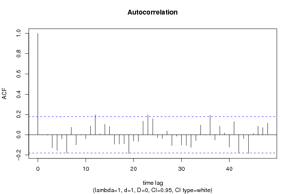
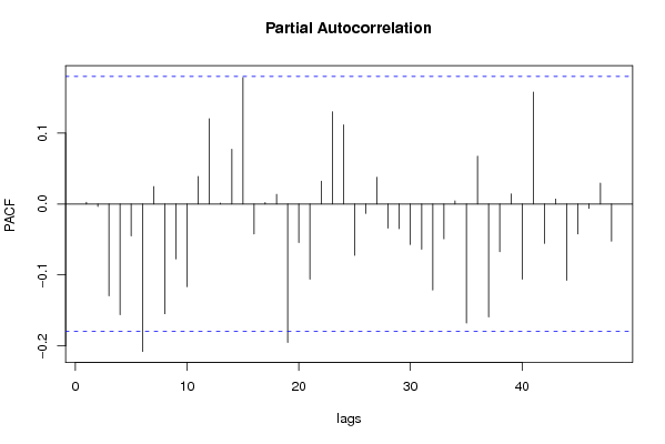
Title produced by software

(Partial) Autocorrelation Function

Date of computation

Sat, 20 Nov 2010 16:45:34 +0000

Cite this page as follows

Statistical Computations at FreeStatistics.org, Office for Research Development and Education, URL https://freestatistics.org/blog/index.php?v=date/2010/Nov/20/t1290271508qp272cq6x4bdzs9.htm/, Retrieved Sat, 27 Apr 2024 11:50:11 +0000

Statistical Computations at FreeStatistics.org, Office for Research Development and Education, URL https://freestatistics.org/blog/index.php?pk=98266, Retrieved Sat, 27 Apr 2024 11:50:11 +0000

QR Codes:

Paste this QR Code to cite your computation.

Original text written by user:

IsPrivate?

No (this computation is public)

User-defined keywords

KDGP2W12

Estimated Impact

121

Family? (F = Feedback message, R = changed R code, M = changed R Module, P = changed Parameters, D = changed Data)

-     [Univariate Data Series] [opgave 6 oef 1] [2010-11-20 12:51:09] [ee977c9178adbf77d0a6da27ad6d4827]
-   PD  [Univariate Data Series] [opgave 6 oef 2] [2010-11-20 13:46:54] [ee977c9178adbf77d0a6da27ad6d4827]
- RMP     [(Partial) Autocorrelation Function] [oef 6 bis oef 2 s...] [2010-11-20 16:28:20] [ee977c9178adbf77d0a6da27ad6d4827]
-    D        [(Partial) Autocorrelation Function] [oef 6 bis oef 2 s...] [2010-11-20 16:45:34] [3c84fba69796ffa9703fc49b6977555d] [Current]

Feedback Forum

Post a new message

Dataseries X:

Download CSV

Histogram

Boxplots

Summary of computational transaction
Raw Input	view raw input (R code)
Raw Output	view raw output of R engine
Computing time	2 seconds
R Server	'RServer@AstonUniversity' @ vre.aston.ac.uk

\begin{tabular}{lllllllll}
\hline
Summary of computational transaction \tabularnewline
Raw Input & view raw input (R code)  \tabularnewline
Raw Output & view raw output of R engine  \tabularnewline
Computing time & 2 seconds \tabularnewline
R Server & 'RServer@AstonUniversity' @ vre.aston.ac.uk \tabularnewline
\hline
\end{tabular}
%Source: https://freestatistics.org/blog/index.php?pk=98266&T=0

[TABLE]
[ROW][C]Summary of computational transaction[/C][/ROW]
[ROW][C]Raw Input[/C][C]view raw input (R code) [/C][/ROW]
[ROW][C]Raw Output[/C][C]view raw output of R engine [/C][/ROW]
[ROW][C]Computing time[/C][C]2 seconds[/C][/ROW]
[ROW][C]R Server[/C][C]'RServer@AstonUniversity' @ vre.aston.ac.uk[/C][/ROW]
[/TABLE]
Source: https://freestatistics.org/blog/index.php?pk=98266&T=0

Globally Unique Identifier (entire table): ba.freestatistics.org/blog/index.php?pk=98266&T=0

As an alternative you can also use a QR Code:

The GUIDs for individual cells are displayed in the table below:

Summary of computational transaction
Raw Input	view raw input (R code)
Raw Output	view raw output of R engine
Computing time	2 seconds
R Server	'RServer@AstonUniversity' @ vre.aston.ac.uk

Autocorrelation Function
Time lag k	ACF(k)	T-STAT	P-value
1	0.002625	0.0286	0.4886
2	-0.003594	-0.0392	0.484397
3	-0.129402	-1.4116	0.080338
4	-0.154044	-1.6804	0.047749
5	-0.039807	-0.4342	0.332449
6	-0.179286	-1.9558	0.026418
7	0.074621	0.814	0.208629
8	-0.099271	-1.0829	0.140516
9	0.001928	0.021	0.491626
10	-0.039932	-0.4356	0.331957
11	0.086824	0.9471	0.172745
12	0.197732	2.157	0.016508
13	0.010011	0.1092	0.456613
14	0.103499	1.129	0.130575
15	0.080151	0.8743	0.191847
16	-0.092293	-1.0068	0.158037
17	-0.091117	-0.994	0.161127
18	-0.090129	-0.9832	0.163753
19	-0.185334	-2.0218	0.022722
20	-0.061474	-0.6706	0.251885
21	-0.066023	-0.7202	0.236399
22	0.134301	1.4651	0.072772
23	0.198362	2.1639	0.016236
24	0.157793	1.7213	0.043896
25	-0.027464	-0.2996	0.382503
26	-0.03717	-0.4055	0.342928
27	0.036886	0.4024	0.344065
28	-0.106342	-1.1601	0.124174
29	-0.013561	-0.1479	0.441324
30	-0.101273	-1.1048	0.135746
31	-0.104615	-1.1412	0.128037
32	-0.124238	-1.3553	0.088949
33	-0.057229	-0.6243	0.266815
34	0.096738	1.0553	0.146716
35	0.003228	0.0352	0.485983
36	0.193371	2.1094	0.018502
37	-0.052319	-0.5707	0.284628
38	0.085901	0.9371	0.175312
39	0.017671	0.1928	0.423733
40	-0.120211	-1.3114	0.096132
41	0.130397	1.4225	0.078754
42	-0.180445	-1.9684	0.025673
43	-0.039199	-0.4276	0.334855
44	-0.183088	-1.9973	0.02404
45	0.013569	0.148	0.441289
46	0.085101	0.9283	0.177554
47	0.071077	0.7754	0.219834
48	0.116117	1.2667	0.103871

\begin{tabular}{lllllllll}
\hline
Autocorrelation Function \tabularnewline
Time lag k & ACF(k) & T-STAT & P-value \tabularnewline
1 & 0.002625 & 0.0286 & 0.4886 \tabularnewline
2 & -0.003594 & -0.0392 & 0.484397 \tabularnewline
3 & -0.129402 & -1.4116 & 0.080338 \tabularnewline
4 & -0.154044 & -1.6804 & 0.047749 \tabularnewline
5 & -0.039807 & -0.4342 & 0.332449 \tabularnewline
6 & -0.179286 & -1.9558 & 0.026418 \tabularnewline
7 & 0.074621 & 0.814 & 0.208629 \tabularnewline
8 & -0.099271 & -1.0829 & 0.140516 \tabularnewline
9 & 0.001928 & 0.021 & 0.491626 \tabularnewline
10 & -0.039932 & -0.4356 & 0.331957 \tabularnewline
11 & 0.086824 & 0.9471 & 0.172745 \tabularnewline
12 & 0.197732 & 2.157 & 0.016508 \tabularnewline
13 & 0.010011 & 0.1092 & 0.456613 \tabularnewline
14 & 0.103499 & 1.129 & 0.130575 \tabularnewline
15 & 0.080151 & 0.8743 & 0.191847 \tabularnewline
16 & -0.092293 & -1.0068 & 0.158037 \tabularnewline
17 & -0.091117 & -0.994 & 0.161127 \tabularnewline
18 & -0.090129 & -0.9832 & 0.163753 \tabularnewline
19 & -0.185334 & -2.0218 & 0.022722 \tabularnewline
20 & -0.061474 & -0.6706 & 0.251885 \tabularnewline
21 & -0.066023 & -0.7202 & 0.236399 \tabularnewline
22 & 0.134301 & 1.4651 & 0.072772 \tabularnewline
23 & 0.198362 & 2.1639 & 0.016236 \tabularnewline
24 & 0.157793 & 1.7213 & 0.043896 \tabularnewline
25 & -0.027464 & -0.2996 & 0.382503 \tabularnewline
26 & -0.03717 & -0.4055 & 0.342928 \tabularnewline
27 & 0.036886 & 0.4024 & 0.344065 \tabularnewline
28 & -0.106342 & -1.1601 & 0.124174 \tabularnewline
29 & -0.013561 & -0.1479 & 0.441324 \tabularnewline
30 & -0.101273 & -1.1048 & 0.135746 \tabularnewline
31 & -0.104615 & -1.1412 & 0.128037 \tabularnewline
32 & -0.124238 & -1.3553 & 0.088949 \tabularnewline
33 & -0.057229 & -0.6243 & 0.266815 \tabularnewline
34 & 0.096738 & 1.0553 & 0.146716 \tabularnewline
35 & 0.003228 & 0.0352 & 0.485983 \tabularnewline
36 & 0.193371 & 2.1094 & 0.018502 \tabularnewline
37 & -0.052319 & -0.5707 & 0.284628 \tabularnewline
38 & 0.085901 & 0.9371 & 0.175312 \tabularnewline
39 & 0.017671 & 0.1928 & 0.423733 \tabularnewline
40 & -0.120211 & -1.3114 & 0.096132 \tabularnewline
41 & 0.130397 & 1.4225 & 0.078754 \tabularnewline
42 & -0.180445 & -1.9684 & 0.025673 \tabularnewline
43 & -0.039199 & -0.4276 & 0.334855 \tabularnewline
44 & -0.183088 & -1.9973 & 0.02404 \tabularnewline
45 & 0.013569 & 0.148 & 0.441289 \tabularnewline
46 & 0.085101 & 0.9283 & 0.177554 \tabularnewline
47 & 0.071077 & 0.7754 & 0.219834 \tabularnewline
48 & 0.116117 & 1.2667 & 0.103871 \tabularnewline
\hline
\end{tabular}
%Source: https://freestatistics.org/blog/index.php?pk=98266&T=1

[TABLE]
[ROW][C]Autocorrelation Function[/C][/ROW]
[ROW][C]Time lag k[/C][C]ACF(k)[/C][C]T-STAT[/C][C]P-value[/C][/ROW]
[ROW][C]1[/C][C]0.002625[/C][C]0.0286[/C][C]0.4886[/C][/ROW]
[ROW][C]2[/C][C]-0.003594[/C][C]-0.0392[/C][C]0.484397[/C][/ROW]
[ROW][C]3[/C][C]-0.129402[/C][C]-1.4116[/C][C]0.080338[/C][/ROW]
[ROW][C]4[/C][C]-0.154044[/C][C]-1.6804[/C][C]0.047749[/C][/ROW]
[ROW][C]5[/C][C]-0.039807[/C][C]-0.4342[/C][C]0.332449[/C][/ROW]
[ROW][C]6[/C][C]-0.179286[/C][C]-1.9558[/C][C]0.026418[/C][/ROW]
[ROW][C]7[/C][C]0.074621[/C][C]0.814[/C][C]0.208629[/C][/ROW]
[ROW][C]8[/C][C]-0.099271[/C][C]-1.0829[/C][C]0.140516[/C][/ROW]
[ROW][C]9[/C][C]0.001928[/C][C]0.021[/C][C]0.491626[/C][/ROW]
[ROW][C]10[/C][C]-0.039932[/C][C]-0.4356[/C][C]0.331957[/C][/ROW]
[ROW][C]11[/C][C]0.086824[/C][C]0.9471[/C][C]0.172745[/C][/ROW]
[ROW][C]12[/C][C]0.197732[/C][C]2.157[/C][C]0.016508[/C][/ROW]
[ROW][C]13[/C][C]0.010011[/C][C]0.1092[/C][C]0.456613[/C][/ROW]
[ROW][C]14[/C][C]0.103499[/C][C]1.129[/C][C]0.130575[/C][/ROW]
[ROW][C]15[/C][C]0.080151[/C][C]0.8743[/C][C]0.191847[/C][/ROW]
[ROW][C]16[/C][C]-0.092293[/C][C]-1.0068[/C][C]0.158037[/C][/ROW]
[ROW][C]17[/C][C]-0.091117[/C][C]-0.994[/C][C]0.161127[/C][/ROW]
[ROW][C]18[/C][C]-0.090129[/C][C]-0.9832[/C][C]0.163753[/C][/ROW]
[ROW][C]19[/C][C]-0.185334[/C][C]-2.0218[/C][C]0.022722[/C][/ROW]
[ROW][C]20[/C][C]-0.061474[/C][C]-0.6706[/C][C]0.251885[/C][/ROW]
[ROW][C]21[/C][C]-0.066023[/C][C]-0.7202[/C][C]0.236399[/C][/ROW]
[ROW][C]22[/C][C]0.134301[/C][C]1.4651[/C][C]0.072772[/C][/ROW]
[ROW][C]23[/C][C]0.198362[/C][C]2.1639[/C][C]0.016236[/C][/ROW]
[ROW][C]24[/C][C]0.157793[/C][C]1.7213[/C][C]0.043896[/C][/ROW]
[ROW][C]25[/C][C]-0.027464[/C][C]-0.2996[/C][C]0.382503[/C][/ROW]
[ROW][C]26[/C][C]-0.03717[/C][C]-0.4055[/C][C]0.342928[/C][/ROW]
[ROW][C]27[/C][C]0.036886[/C][C]0.4024[/C][C]0.344065[/C][/ROW]
[ROW][C]28[/C][C]-0.106342[/C][C]-1.1601[/C][C]0.124174[/C][/ROW]
[ROW][C]29[/C][C]-0.013561[/C][C]-0.1479[/C][C]0.441324[/C][/ROW]
[ROW][C]30[/C][C]-0.101273[/C][C]-1.1048[/C][C]0.135746[/C][/ROW]
[ROW][C]31[/C][C]-0.104615[/C][C]-1.1412[/C][C]0.128037[/C][/ROW]
[ROW][C]32[/C][C]-0.124238[/C][C]-1.3553[/C][C]0.088949[/C][/ROW]
[ROW][C]33[/C][C]-0.057229[/C][C]-0.6243[/C][C]0.266815[/C][/ROW]
[ROW][C]34[/C][C]0.096738[/C][C]1.0553[/C][C]0.146716[/C][/ROW]
[ROW][C]35[/C][C]0.003228[/C][C]0.0352[/C][C]0.485983[/C][/ROW]
[ROW][C]36[/C][C]0.193371[/C][C]2.1094[/C][C]0.018502[/C][/ROW]
[ROW][C]37[/C][C]-0.052319[/C][C]-0.5707[/C][C]0.284628[/C][/ROW]
[ROW][C]38[/C][C]0.085901[/C][C]0.9371[/C][C]0.175312[/C][/ROW]
[ROW][C]39[/C][C]0.017671[/C][C]0.1928[/C][C]0.423733[/C][/ROW]
[ROW][C]40[/C][C]-0.120211[/C][C]-1.3114[/C][C]0.096132[/C][/ROW]
[ROW][C]41[/C][C]0.130397[/C][C]1.4225[/C][C]0.078754[/C][/ROW]
[ROW][C]42[/C][C]-0.180445[/C][C]-1.9684[/C][C]0.025673[/C][/ROW]
[ROW][C]43[/C][C]-0.039199[/C][C]-0.4276[/C][C]0.334855[/C][/ROW]
[ROW][C]44[/C][C]-0.183088[/C][C]-1.9973[/C][C]0.02404[/C][/ROW]
[ROW][C]45[/C][C]0.013569[/C][C]0.148[/C][C]0.441289[/C][/ROW]
[ROW][C]46[/C][C]0.085101[/C][C]0.9283[/C][C]0.177554[/C][/ROW]
[ROW][C]47[/C][C]0.071077[/C][C]0.7754[/C][C]0.219834[/C][/ROW]
[ROW][C]48[/C][C]0.116117[/C][C]1.2667[/C][C]0.103871[/C][/ROW]
[/TABLE]
Source: https://freestatistics.org/blog/index.php?pk=98266&T=1

Globally Unique Identifier (entire table): ba.freestatistics.org/blog/index.php?pk=98266&T=1

As an alternative you can also use a QR Code:

The GUIDs for individual cells are displayed in the table below:

Autocorrelation Function
Time lag k	ACF(k)	T-STAT	P-value
1	0.002625	0.0286	0.4886
2	-0.003594	-0.0392	0.484397
3	-0.129402	-1.4116	0.080338
4	-0.154044	-1.6804	0.047749
5	-0.039807	-0.4342	0.332449
6	-0.179286	-1.9558	0.026418
7	0.074621	0.814	0.208629
8	-0.099271	-1.0829	0.140516
9	0.001928	0.021	0.491626
10	-0.039932	-0.4356	0.331957
11	0.086824	0.9471	0.172745
12	0.197732	2.157	0.016508
13	0.010011	0.1092	0.456613
14	0.103499	1.129	0.130575
15	0.080151	0.8743	0.191847
16	-0.092293	-1.0068	0.158037
17	-0.091117	-0.994	0.161127
18	-0.090129	-0.9832	0.163753
19	-0.185334	-2.0218	0.022722
20	-0.061474	-0.6706	0.251885
21	-0.066023	-0.7202	0.236399
22	0.134301	1.4651	0.072772
23	0.198362	2.1639	0.016236
24	0.157793	1.7213	0.043896
25	-0.027464	-0.2996	0.382503
26	-0.03717	-0.4055	0.342928
27	0.036886	0.4024	0.344065
28	-0.106342	-1.1601	0.124174
29	-0.013561	-0.1479	0.441324
30	-0.101273	-1.1048	0.135746
31	-0.104615	-1.1412	0.128037
32	-0.124238	-1.3553	0.088949
33	-0.057229	-0.6243	0.266815
34	0.096738	1.0553	0.146716
35	0.003228	0.0352	0.485983
36	0.193371	2.1094	0.018502
37	-0.052319	-0.5707	0.284628
38	0.085901	0.9371	0.175312
39	0.017671	0.1928	0.423733
40	-0.120211	-1.3114	0.096132
41	0.130397	1.4225	0.078754
42	-0.180445	-1.9684	0.025673
43	-0.039199	-0.4276	0.334855
44	-0.183088	-1.9973	0.02404
45	0.013569	0.148	0.441289
46	0.085101	0.9283	0.177554
47	0.071077	0.7754	0.219834
48	0.116117	1.2667	0.103871

Partial Autocorrelation Function
Time lag k	PACF(k)	T-STAT	P-value
1	0.002625	0.0286	0.4886
2	-0.003601	-0.0393	0.484367
3	-0.129385	-1.4114	0.080364
4	-0.156051	-1.7023	0.045654
5	-0.044955	-0.4904	0.312378
6	-0.207783	-2.2666	0.012609
7	0.024616	0.2685	0.394379
8	-0.154592	-1.6864	0.047169
9	-0.077475	-0.8452	0.199861
10	-0.116613	-1.2721	0.10291
11	0.038949	0.4249	0.335846
12	0.120322	1.3126	0.09593
13	0.001429	0.0156	0.493796
14	0.077037	0.8404	0.201192
15	0.178285	1.9449	0.027076
16	-0.042222	-0.4606	0.322968
17	0.002011	0.0219	0.491268
18	0.013635	0.1487	0.441004
19	-0.194976	-2.1269	0.017745
20	-0.054363	-0.593	0.277144
21	-0.105939	-1.1557	0.125067
22	0.032357	0.353	0.362366
23	0.129939	1.4175	0.079479
24	0.111731	1.2188	0.112658
25	-0.072183	-0.7874	0.216299
26	-0.01328	-0.1449	0.442529
27	0.037758	0.4119	0.340578
28	-0.033998	-0.3709	0.355696
29	-0.034656	-0.3781	0.353033
30	-0.057092	-0.6228	0.267303
31	-0.06378	-0.6958	0.243969
32	-0.121051	-1.3205	0.0946
33	-0.048981	-0.5343	0.297057
34	0.00435	0.0475	0.481115
35	-0.167599	-1.8283	0.035006
36	0.06745	0.7358	0.231651
37	-0.159201	-1.7367	0.042516
38	-0.06712	-0.7322	0.232746
39	0.014184	0.1547	0.438647
40	-0.10598	-1.1561	0.124977
41	0.157777	1.7211	0.043912
42	-0.055348	-0.6038	0.273572
43	0.006954	0.0759	0.469831
44	-0.107448	-1.1721	0.121746
45	-0.042302	-0.4615	0.322656
46	-0.006268	-0.0684	0.472803
47	0.029578	0.3227	0.37376
48	-0.052274	-0.5702	0.284795

\begin{tabular}{lllllllll}
\hline
Partial Autocorrelation Function \tabularnewline
Time lag k & PACF(k) & T-STAT & P-value \tabularnewline
1 & 0.002625 & 0.0286 & 0.4886 \tabularnewline
2 & -0.003601 & -0.0393 & 0.484367 \tabularnewline
3 & -0.129385 & -1.4114 & 0.080364 \tabularnewline
4 & -0.156051 & -1.7023 & 0.045654 \tabularnewline
5 & -0.044955 & -0.4904 & 0.312378 \tabularnewline
6 & -0.207783 & -2.2666 & 0.012609 \tabularnewline
7 & 0.024616 & 0.2685 & 0.394379 \tabularnewline
8 & -0.154592 & -1.6864 & 0.047169 \tabularnewline
9 & -0.077475 & -0.8452 & 0.199861 \tabularnewline
10 & -0.116613 & -1.2721 & 0.10291 \tabularnewline
11 & 0.038949 & 0.4249 & 0.335846 \tabularnewline
12 & 0.120322 & 1.3126 & 0.09593 \tabularnewline
13 & 0.001429 & 0.0156 & 0.493796 \tabularnewline
14 & 0.077037 & 0.8404 & 0.201192 \tabularnewline
15 & 0.178285 & 1.9449 & 0.027076 \tabularnewline
16 & -0.042222 & -0.4606 & 0.322968 \tabularnewline
17 & 0.002011 & 0.0219 & 0.491268 \tabularnewline
18 & 0.013635 & 0.1487 & 0.441004 \tabularnewline
19 & -0.194976 & -2.1269 & 0.017745 \tabularnewline
20 & -0.054363 & -0.593 & 0.277144 \tabularnewline
21 & -0.105939 & -1.1557 & 0.125067 \tabularnewline
22 & 0.032357 & 0.353 & 0.362366 \tabularnewline
23 & 0.129939 & 1.4175 & 0.079479 \tabularnewline
24 & 0.111731 & 1.2188 & 0.112658 \tabularnewline
25 & -0.072183 & -0.7874 & 0.216299 \tabularnewline
26 & -0.01328 & -0.1449 & 0.442529 \tabularnewline
27 & 0.037758 & 0.4119 & 0.340578 \tabularnewline
28 & -0.033998 & -0.3709 & 0.355696 \tabularnewline
29 & -0.034656 & -0.3781 & 0.353033 \tabularnewline
30 & -0.057092 & -0.6228 & 0.267303 \tabularnewline
31 & -0.06378 & -0.6958 & 0.243969 \tabularnewline
32 & -0.121051 & -1.3205 & 0.0946 \tabularnewline
33 & -0.048981 & -0.5343 & 0.297057 \tabularnewline
34 & 0.00435 & 0.0475 & 0.481115 \tabularnewline
35 & -0.167599 & -1.8283 & 0.035006 \tabularnewline
36 & 0.06745 & 0.7358 & 0.231651 \tabularnewline
37 & -0.159201 & -1.7367 & 0.042516 \tabularnewline
38 & -0.06712 & -0.7322 & 0.232746 \tabularnewline
39 & 0.014184 & 0.1547 & 0.438647 \tabularnewline
40 & -0.10598 & -1.1561 & 0.124977 \tabularnewline
41 & 0.157777 & 1.7211 & 0.043912 \tabularnewline
42 & -0.055348 & -0.6038 & 0.273572 \tabularnewline
43 & 0.006954 & 0.0759 & 0.469831 \tabularnewline
44 & -0.107448 & -1.1721 & 0.121746 \tabularnewline
45 & -0.042302 & -0.4615 & 0.322656 \tabularnewline
46 & -0.006268 & -0.0684 & 0.472803 \tabularnewline
47 & 0.029578 & 0.3227 & 0.37376 \tabularnewline
48 & -0.052274 & -0.5702 & 0.284795 \tabularnewline
\hline
\end{tabular}
%Source: https://freestatistics.org/blog/index.php?pk=98266&T=2

[TABLE]
[ROW][C]Partial Autocorrelation Function[/C][/ROW]
[ROW][C]Time lag k[/C][C]PACF(k)[/C][C]T-STAT[/C][C]P-value[/C][/ROW]
[ROW][C]1[/C][C]0.002625[/C][C]0.0286[/C][C]0.4886[/C][/ROW]
[ROW][C]2[/C][C]-0.003601[/C][C]-0.0393[/C][C]0.484367[/C][/ROW]
[ROW][C]3[/C][C]-0.129385[/C][C]-1.4114[/C][C]0.080364[/C][/ROW]
[ROW][C]4[/C][C]-0.156051[/C][C]-1.7023[/C][C]0.045654[/C][/ROW]
[ROW][C]5[/C][C]-0.044955[/C][C]-0.4904[/C][C]0.312378[/C][/ROW]
[ROW][C]6[/C][C]-0.207783[/C][C]-2.2666[/C][C]0.012609[/C][/ROW]
[ROW][C]7[/C][C]0.024616[/C][C]0.2685[/C][C]0.394379[/C][/ROW]
[ROW][C]8[/C][C]-0.154592[/C][C]-1.6864[/C][C]0.047169[/C][/ROW]
[ROW][C]9[/C][C]-0.077475[/C][C]-0.8452[/C][C]0.199861[/C][/ROW]
[ROW][C]10[/C][C]-0.116613[/C][C]-1.2721[/C][C]0.10291[/C][/ROW]
[ROW][C]11[/C][C]0.038949[/C][C]0.4249[/C][C]0.335846[/C][/ROW]
[ROW][C]12[/C][C]0.120322[/C][C]1.3126[/C][C]0.09593[/C][/ROW]
[ROW][C]13[/C][C]0.001429[/C][C]0.0156[/C][C]0.493796[/C][/ROW]
[ROW][C]14[/C][C]0.077037[/C][C]0.8404[/C][C]0.201192[/C][/ROW]
[ROW][C]15[/C][C]0.178285[/C][C]1.9449[/C][C]0.027076[/C][/ROW]
[ROW][C]16[/C][C]-0.042222[/C][C]-0.4606[/C][C]0.322968[/C][/ROW]
[ROW][C]17[/C][C]0.002011[/C][C]0.0219[/C][C]0.491268[/C][/ROW]
[ROW][C]18[/C][C]0.013635[/C][C]0.1487[/C][C]0.441004[/C][/ROW]
[ROW][C]19[/C][C]-0.194976[/C][C]-2.1269[/C][C]0.017745[/C][/ROW]
[ROW][C]20[/C][C]-0.054363[/C][C]-0.593[/C][C]0.277144[/C][/ROW]
[ROW][C]21[/C][C]-0.105939[/C][C]-1.1557[/C][C]0.125067[/C][/ROW]
[ROW][C]22[/C][C]0.032357[/C][C]0.353[/C][C]0.362366[/C][/ROW]
[ROW][C]23[/C][C]0.129939[/C][C]1.4175[/C][C]0.079479[/C][/ROW]
[ROW][C]24[/C][C]0.111731[/C][C]1.2188[/C][C]0.112658[/C][/ROW]
[ROW][C]25[/C][C]-0.072183[/C][C]-0.7874[/C][C]0.216299[/C][/ROW]
[ROW][C]26[/C][C]-0.01328[/C][C]-0.1449[/C][C]0.442529[/C][/ROW]
[ROW][C]27[/C][C]0.037758[/C][C]0.4119[/C][C]0.340578[/C][/ROW]
[ROW][C]28[/C][C]-0.033998[/C][C]-0.3709[/C][C]0.355696[/C][/ROW]
[ROW][C]29[/C][C]-0.034656[/C][C]-0.3781[/C][C]0.353033[/C][/ROW]
[ROW][C]30[/C][C]-0.057092[/C][C]-0.6228[/C][C]0.267303[/C][/ROW]
[ROW][C]31[/C][C]-0.06378[/C][C]-0.6958[/C][C]0.243969[/C][/ROW]
[ROW][C]32[/C][C]-0.121051[/C][C]-1.3205[/C][C]0.0946[/C][/ROW]
[ROW][C]33[/C][C]-0.048981[/C][C]-0.5343[/C][C]0.297057[/C][/ROW]
[ROW][C]34[/C][C]0.00435[/C][C]0.0475[/C][C]0.481115[/C][/ROW]
[ROW][C]35[/C][C]-0.167599[/C][C]-1.8283[/C][C]0.035006[/C][/ROW]
[ROW][C]36[/C][C]0.06745[/C][C]0.7358[/C][C]0.231651[/C][/ROW]
[ROW][C]37[/C][C]-0.159201[/C][C]-1.7367[/C][C]0.042516[/C][/ROW]
[ROW][C]38[/C][C]-0.06712[/C][C]-0.7322[/C][C]0.232746[/C][/ROW]
[ROW][C]39[/C][C]0.014184[/C][C]0.1547[/C][C]0.438647[/C][/ROW]
[ROW][C]40[/C][C]-0.10598[/C][C]-1.1561[/C][C]0.124977[/C][/ROW]
[ROW][C]41[/C][C]0.157777[/C][C]1.7211[/C][C]0.043912[/C][/ROW]
[ROW][C]42[/C][C]-0.055348[/C][C]-0.6038[/C][C]0.273572[/C][/ROW]
[ROW][C]43[/C][C]0.006954[/C][C]0.0759[/C][C]0.469831[/C][/ROW]
[ROW][C]44[/C][C]-0.107448[/C][C]-1.1721[/C][C]0.121746[/C][/ROW]
[ROW][C]45[/C][C]-0.042302[/C][C]-0.4615[/C][C]0.322656[/C][/ROW]
[ROW][C]46[/C][C]-0.006268[/C][C]-0.0684[/C][C]0.472803[/C][/ROW]
[ROW][C]47[/C][C]0.029578[/C][C]0.3227[/C][C]0.37376[/C][/ROW]
[ROW][C]48[/C][C]-0.052274[/C][C]-0.5702[/C][C]0.284795[/C][/ROW]
[/TABLE]
Source: https://freestatistics.org/blog/index.php?pk=98266&T=2

Globally Unique Identifier (entire table): ba.freestatistics.org/blog/index.php?pk=98266&T=2

As an alternative you can also use a QR Code:

The GUIDs for individual cells are displayed in the table below:

Partial Autocorrelation Function
Time lag k	PACF(k)	T-STAT	P-value
1	0.002625	0.0286	0.4886
2	-0.003601	-0.0393	0.484367
3	-0.129385	-1.4114	0.080364
4	-0.156051	-1.7023	0.045654
5	-0.044955	-0.4904	0.312378
6	-0.207783	-2.2666	0.012609
7	0.024616	0.2685	0.394379
8	-0.154592	-1.6864	0.047169
9	-0.077475	-0.8452	0.199861
10	-0.116613	-1.2721	0.10291
11	0.038949	0.4249	0.335846
12	0.120322	1.3126	0.09593
13	0.001429	0.0156	0.493796
14	0.077037	0.8404	0.201192
15	0.178285	1.9449	0.027076
16	-0.042222	-0.4606	0.322968
17	0.002011	0.0219	0.491268
18	0.013635	0.1487	0.441004
19	-0.194976	-2.1269	0.017745
20	-0.054363	-0.593	0.277144
21	-0.105939	-1.1557	0.125067
22	0.032357	0.353	0.362366
23	0.129939	1.4175	0.079479
24	0.111731	1.2188	0.112658
25	-0.072183	-0.7874	0.216299
26	-0.01328	-0.1449	0.442529
27	0.037758	0.4119	0.340578
28	-0.033998	-0.3709	0.355696
29	-0.034656	-0.3781	0.353033
30	-0.057092	-0.6228	0.267303
31	-0.06378	-0.6958	0.243969
32	-0.121051	-1.3205	0.0946
33	-0.048981	-0.5343	0.297057
34	0.00435	0.0475	0.481115
35	-0.167599	-1.8283	0.035006
36	0.06745	0.7358	0.231651
37	-0.159201	-1.7367	0.042516
38	-0.06712	-0.7322	0.232746
39	0.014184	0.1547	0.438647
40	-0.10598	-1.1561	0.124977
41	0.157777	1.7211	0.043912
42	-0.055348	-0.6038	0.273572
43	0.006954	0.0759	0.469831
44	-0.107448	-1.1721	0.121746
45	-0.042302	-0.4615	0.322656
46	-0.006268	-0.0684	0.472803
47	0.029578	0.3227	0.37376
48	-0.052274	-0.5702	0.284795

Figure 1

PNG link

Postscript link

PDF link

Figure 2

PNG link

Postscript link

PDF link

Parameters (Session):

par1 = 48 ; par2 = 1 ; par3 = 1 ; par4 = 0 ; par5 = 12 ; par6 = White Noise ; par7 = 0.95 ;

Parameters (R input):

par1 = 48 ; par2 = 1 ; par3 = 1 ; par4 = 0 ; par5 = 12 ; par6 = White Noise ; par7 = 0.95 ;

R code (references can be found in the software module):

if (par1 == 'Default') {
par1 = 10*log10(length(x))
} else {
par1 <- as.numeric(par1)
}
par2 <- as.numeric(par2)
par3 <- as.numeric(par3)
par4 <- as.numeric(par4)
par5 <- as.numeric(par5)
if (par6 == 'White Noise') par6 <- 'white' else par6 <- 'ma'
par7 <- as.numeric(par7)
if (par2 == 0) {
x <- log(x)
} else {
x <- (x ^ par2 - 1) / par2
}
if (par3 > 0) x <- diff(x,lag=1,difference=par3)
if (par4 > 0) x <- diff(x,lag=par5,difference=par4)
bitmap(file='pic1.png')
racf <- acf(x, par1, main='Autocorrelation', xlab='time lag', ylab='ACF', ci.type=par6, ci=par7, sub=paste('(lambda=',par2,', d=',par3,', D=',par4,', CI=', par7, ', CI type=',par6,')',sep=''))
dev.off()
bitmap(file='pic2.png')
rpacf <- pacf(x,par1,main='Partial Autocorrelation',xlab='lags',ylab='PACF')
dev.off()
(myacf <- c(racf$acf))
(mypacf <- c(rpacf$acf))
lengthx <- length(x)
sqrtn <- sqrt(lengthx)
load(file='createtable')
a<-table.start()
a<-table.row.start(a)
a<-table.element(a,'Autocorrelation Function',4,TRUE)
a<-table.row.end(a)
a<-table.row.start(a)
a<-table.element(a,'Time lag k',header=TRUE)
a<-table.element(a,hyperlink('basics.htm','ACF(k)','click here for more information about the Autocorrelation Function'),header=TRUE)
a<-table.element(a,'T-STAT',header=TRUE)
a<-table.element(a,'P-value',header=TRUE)
a<-table.row.end(a)
for (i in 2:(par1+1)) {
a<-table.row.start(a)
a<-table.element(a,i-1,header=TRUE)
a<-table.element(a,round(myacf[i],6))
mytstat <- myacf[i]*sqrtn
a<-table.element(a,round(mytstat,4))
a<-table.element(a,round(1-pt(abs(mytstat),lengthx),6))
a<-table.row.end(a)
}
a<-table.end(a)
table.save(a,file='mytable.tab')
a<-table.start()
a<-table.row.start(a)
a<-table.element(a,'Partial Autocorrelation Function',4,TRUE)
a<-table.row.end(a)
a<-table.row.start(a)
a<-table.element(a,'Time lag k',header=TRUE)
a<-table.element(a,hyperlink('basics.htm','PACF(k)','click here for more information about the Partial Autocorrelation Function'),header=TRUE)
a<-table.element(a,'T-STAT',header=TRUE)
a<-table.element(a,'P-value',header=TRUE)
a<-table.row.end(a)
for (i in 1:par1) {
a<-table.row.start(a)
a<-table.element(a,i,header=TRUE)
a<-table.element(a,round(mypacf[i],6))
mytstat <- mypacf[i]*sqrtn
a<-table.element(a,round(mytstat,4))
a<-table.element(a,round(1-pt(abs(mytstat),lengthx),6))
a<-table.row.end(a)
}
a<-table.end(a)
table.save(a,file='mytable1.tab')

Free Statistics

Description of Statistical Computation

Tree of Dependent Computations

Dataset

Tables (Output of Computation)

Figures (Output of Computation)

Input Parameters & R Code