Repository of Reproducible Computations

Free Statistics

of Irreproducible Research!

Author's title

Author

*Unverified author*

R Software Module

rwasp_autocorrelation.wasp

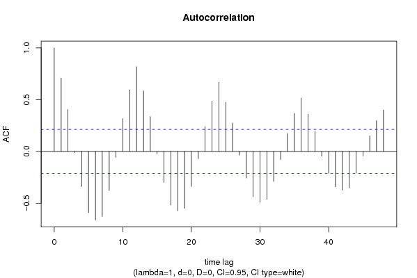
Title produced by software

(Partial) Autocorrelation Function

Date of computation

Wed, 17 Nov 2010 20:36:20 +0000

Cite this page as follows

Statistical Computations at FreeStatistics.org, Office for Research Development and Education, URL https://freestatistics.org/blog/index.php?v=date/2010/Nov/17/t12900261927gn5oyxgy5tc003.htm/, Retrieved Fri, 19 Apr 2024 15:43:01 +0000

Statistical Computations at FreeStatistics.org, Office for Research Development and Education, URL https://freestatistics.org/blog/index.php?pk=96939, Retrieved Fri, 19 Apr 2024 15:43:01 +0000

QR Codes:

Paste this QR Code to cite your computation.

Original text written by user:

IsPrivate?

No (this computation is public)

User-defined keywords

KDGP2W12

Estimated Impact

119

Family? (F = Feedback message, R = changed R code, M = changed R Module, P = changed Parameters, D = changed Data)

-       [(Partial) Autocorrelation Function] [opg6bis_deel2] [2010-11-17 20:36:20] [ba6a6eaac02e80e5d4f1379a58894c63] [Current]

Feedback Forum

Post a new message

Dataseries X:

Download CSV

Histogram

Boxplots

Summary of computational transaction
Raw Input	view raw input (R code)
Raw Output	view raw output of R engine
Computing time	2 seconds
R Server	'Gwilym Jenkins' @ 72.249.127.135

\begin{tabular}{lllllllll}
\hline
Summary of computational transaction \tabularnewline
Raw Input & view raw input (R code)  \tabularnewline
Raw Output & view raw output of R engine  \tabularnewline
Computing time & 2 seconds \tabularnewline
R Server & 'Gwilym Jenkins' @ 72.249.127.135 \tabularnewline
\hline
\end{tabular}
%Source: https://freestatistics.org/blog/index.php?pk=96939&T=0

[TABLE]
[ROW][C]Summary of computational transaction[/C][/ROW]
[ROW][C]Raw Input[/C][C]view raw input (R code) [/C][/ROW]
[ROW][C]Raw Output[/C][C]view raw output of R engine [/C][/ROW]
[ROW][C]Computing time[/C][C]2 seconds[/C][/ROW]
[ROW][C]R Server[/C][C]'Gwilym Jenkins' @ 72.249.127.135[/C][/ROW]
[/TABLE]
Source: https://freestatistics.org/blog/index.php?pk=96939&T=0

Globally Unique Identifier (entire table): ba.freestatistics.org/blog/index.php?pk=96939&T=0

As an alternative you can also use a QR Code:

The GUIDs for individual cells are displayed in the table below:

Summary of computational transaction
Raw Input	view raw input (R code)
Raw Output	view raw output of R engine
Computing time	2 seconds
R Server	'Gwilym Jenkins' @ 72.249.127.135

Autocorrelation Function
Time lag k	ACF(k)	T-STAT	P-value
1	0.710033	6.5076	0
2	0.405198	3.7137	0.000183
3	-0.011264	-0.1032	0.459011
4	-0.338724	-3.1045	0.001299
5	-0.592951	-5.4345	0
6	-0.663109	-6.0775	0
7	-0.628773	-5.7628	0
8	-0.377797	-3.4626	0.000422
9	-0.057725	-0.5291	0.29908
10	0.318015	2.9147	0.002282
11	0.595228	5.4554	0
12	0.818544	7.5021	0
13	0.585549	5.3666	0
14	0.336226	3.0816	0.001392
15	-0.021991	-0.2016	0.420376
16	-0.299672	-2.7465	0.003684
17	-0.518078	-4.7483	4e-06
18	-0.575033	-5.2703	1e-06
19	-0.550093	-5.0417	1e-06
20	-0.338402	-3.1015	0.001311
21	-0.070329	-0.6446	0.260479
22	0.240355	2.2029	0.01517
23	0.486125	4.4554	1.3e-05
24	0.66928	6.1341	0
25	0.475706	4.3599	1.8e-05
26	0.274463	2.5155	0.006895
27	-0.035381	-0.3243	0.373269
28	-0.256208	-2.3482	0.010608
29	-0.437087	-4.006	6.6e-05
30	-0.490975	-4.4999	1.1e-05
31	-0.46394	-4.2521	2.7e-05
32	-0.288897	-2.6478	0.004837
33	-0.077639	-0.7116	0.23935
34	0.173409	1.5893	0.057873
35	0.367348	3.3668	0.000575
36	0.516853	4.737	4e-06
37	0.360097	3.3003	0.000709
38	0.192372	1.7631	0.040759
39	-0.045625	-0.4182	0.338449
40	-0.211713	-1.9404	0.027844
41	-0.340789	-3.1234	0.001227
42	-0.375085	-3.4377	0.000457
43	-0.353256	-3.2376	0.000863
44	-0.208267	-1.9088	0.029851
45	-0.04206	-0.3855	0.350427
46	0.15069	1.3811	0.085456
47	0.298026	2.7315	0.003842
48	0.40101	3.6753	0.000209

\begin{tabular}{lllllllll}
\hline
Autocorrelation Function \tabularnewline
Time lag k & ACF(k) & T-STAT & P-value \tabularnewline
1 & 0.710033 & 6.5076 & 0 \tabularnewline
2 & 0.405198 & 3.7137 & 0.000183 \tabularnewline
3 & -0.011264 & -0.1032 & 0.459011 \tabularnewline
4 & -0.338724 & -3.1045 & 0.001299 \tabularnewline
5 & -0.592951 & -5.4345 & 0 \tabularnewline
6 & -0.663109 & -6.0775 & 0 \tabularnewline
7 & -0.628773 & -5.7628 & 0 \tabularnewline
8 & -0.377797 & -3.4626 & 0.000422 \tabularnewline
9 & -0.057725 & -0.5291 & 0.29908 \tabularnewline
10 & 0.318015 & 2.9147 & 0.002282 \tabularnewline
11 & 0.595228 & 5.4554 & 0 \tabularnewline
12 & 0.818544 & 7.5021 & 0 \tabularnewline
13 & 0.585549 & 5.3666 & 0 \tabularnewline
14 & 0.336226 & 3.0816 & 0.001392 \tabularnewline
15 & -0.021991 & -0.2016 & 0.420376 \tabularnewline
16 & -0.299672 & -2.7465 & 0.003684 \tabularnewline
17 & -0.518078 & -4.7483 & 4e-06 \tabularnewline
18 & -0.575033 & -5.2703 & 1e-06 \tabularnewline
19 & -0.550093 & -5.0417 & 1e-06 \tabularnewline
20 & -0.338402 & -3.1015 & 0.001311 \tabularnewline
21 & -0.070329 & -0.6446 & 0.260479 \tabularnewline
22 & 0.240355 & 2.2029 & 0.01517 \tabularnewline
23 & 0.486125 & 4.4554 & 1.3e-05 \tabularnewline
24 & 0.66928 & 6.1341 & 0 \tabularnewline
25 & 0.475706 & 4.3599 & 1.8e-05 \tabularnewline
26 & 0.274463 & 2.5155 & 0.006895 \tabularnewline
27 & -0.035381 & -0.3243 & 0.373269 \tabularnewline
28 & -0.256208 & -2.3482 & 0.010608 \tabularnewline
29 & -0.437087 & -4.006 & 6.6e-05 \tabularnewline
30 & -0.490975 & -4.4999 & 1.1e-05 \tabularnewline
31 & -0.46394 & -4.2521 & 2.7e-05 \tabularnewline
32 & -0.288897 & -2.6478 & 0.004837 \tabularnewline
33 & -0.077639 & -0.7116 & 0.23935 \tabularnewline
34 & 0.173409 & 1.5893 & 0.057873 \tabularnewline
35 & 0.367348 & 3.3668 & 0.000575 \tabularnewline
36 & 0.516853 & 4.737 & 4e-06 \tabularnewline
37 & 0.360097 & 3.3003 & 0.000709 \tabularnewline
38 & 0.192372 & 1.7631 & 0.040759 \tabularnewline
39 & -0.045625 & -0.4182 & 0.338449 \tabularnewline
40 & -0.211713 & -1.9404 & 0.027844 \tabularnewline
41 & -0.340789 & -3.1234 & 0.001227 \tabularnewline
42 & -0.375085 & -3.4377 & 0.000457 \tabularnewline
43 & -0.353256 & -3.2376 & 0.000863 \tabularnewline
44 & -0.208267 & -1.9088 & 0.029851 \tabularnewline
45 & -0.04206 & -0.3855 & 0.350427 \tabularnewline
46 & 0.15069 & 1.3811 & 0.085456 \tabularnewline
47 & 0.298026 & 2.7315 & 0.003842 \tabularnewline
48 & 0.40101 & 3.6753 & 0.000209 \tabularnewline
\hline
\end{tabular}
%Source: https://freestatistics.org/blog/index.php?pk=96939&T=1

[TABLE]
[ROW][C]Autocorrelation Function[/C][/ROW]
[ROW][C]Time lag k[/C][C]ACF(k)[/C][C]T-STAT[/C][C]P-value[/C][/ROW]
[ROW][C]1[/C][C]0.710033[/C][C]6.5076[/C][C]0[/C][/ROW]
[ROW][C]2[/C][C]0.405198[/C][C]3.7137[/C][C]0.000183[/C][/ROW]
[ROW][C]3[/C][C]-0.011264[/C][C]-0.1032[/C][C]0.459011[/C][/ROW]
[ROW][C]4[/C][C]-0.338724[/C][C]-3.1045[/C][C]0.001299[/C][/ROW]
[ROW][C]5[/C][C]-0.592951[/C][C]-5.4345[/C][C]0[/C][/ROW]
[ROW][C]6[/C][C]-0.663109[/C][C]-6.0775[/C][C]0[/C][/ROW]
[ROW][C]7[/C][C]-0.628773[/C][C]-5.7628[/C][C]0[/C][/ROW]
[ROW][C]8[/C][C]-0.377797[/C][C]-3.4626[/C][C]0.000422[/C][/ROW]
[ROW][C]9[/C][C]-0.057725[/C][C]-0.5291[/C][C]0.29908[/C][/ROW]
[ROW][C]10[/C][C]0.318015[/C][C]2.9147[/C][C]0.002282[/C][/ROW]
[ROW][C]11[/C][C]0.595228[/C][C]5.4554[/C][C]0[/C][/ROW]
[ROW][C]12[/C][C]0.818544[/C][C]7.5021[/C][C]0[/C][/ROW]
[ROW][C]13[/C][C]0.585549[/C][C]5.3666[/C][C]0[/C][/ROW]
[ROW][C]14[/C][C]0.336226[/C][C]3.0816[/C][C]0.001392[/C][/ROW]
[ROW][C]15[/C][C]-0.021991[/C][C]-0.2016[/C][C]0.420376[/C][/ROW]
[ROW][C]16[/C][C]-0.299672[/C][C]-2.7465[/C][C]0.003684[/C][/ROW]
[ROW][C]17[/C][C]-0.518078[/C][C]-4.7483[/C][C]4e-06[/C][/ROW]
[ROW][C]18[/C][C]-0.575033[/C][C]-5.2703[/C][C]1e-06[/C][/ROW]
[ROW][C]19[/C][C]-0.550093[/C][C]-5.0417[/C][C]1e-06[/C][/ROW]
[ROW][C]20[/C][C]-0.338402[/C][C]-3.1015[/C][C]0.001311[/C][/ROW]
[ROW][C]21[/C][C]-0.070329[/C][C]-0.6446[/C][C]0.260479[/C][/ROW]
[ROW][C]22[/C][C]0.240355[/C][C]2.2029[/C][C]0.01517[/C][/ROW]
[ROW][C]23[/C][C]0.486125[/C][C]4.4554[/C][C]1.3e-05[/C][/ROW]
[ROW][C]24[/C][C]0.66928[/C][C]6.1341[/C][C]0[/C][/ROW]
[ROW][C]25[/C][C]0.475706[/C][C]4.3599[/C][C]1.8e-05[/C][/ROW]
[ROW][C]26[/C][C]0.274463[/C][C]2.5155[/C][C]0.006895[/C][/ROW]
[ROW][C]27[/C][C]-0.035381[/C][C]-0.3243[/C][C]0.373269[/C][/ROW]
[ROW][C]28[/C][C]-0.256208[/C][C]-2.3482[/C][C]0.010608[/C][/ROW]
[ROW][C]29[/C][C]-0.437087[/C][C]-4.006[/C][C]6.6e-05[/C][/ROW]
[ROW][C]30[/C][C]-0.490975[/C][C]-4.4999[/C][C]1.1e-05[/C][/ROW]
[ROW][C]31[/C][C]-0.46394[/C][C]-4.2521[/C][C]2.7e-05[/C][/ROW]
[ROW][C]32[/C][C]-0.288897[/C][C]-2.6478[/C][C]0.004837[/C][/ROW]
[ROW][C]33[/C][C]-0.077639[/C][C]-0.7116[/C][C]0.23935[/C][/ROW]
[ROW][C]34[/C][C]0.173409[/C][C]1.5893[/C][C]0.057873[/C][/ROW]
[ROW][C]35[/C][C]0.367348[/C][C]3.3668[/C][C]0.000575[/C][/ROW]
[ROW][C]36[/C][C]0.516853[/C][C]4.737[/C][C]4e-06[/C][/ROW]
[ROW][C]37[/C][C]0.360097[/C][C]3.3003[/C][C]0.000709[/C][/ROW]
[ROW][C]38[/C][C]0.192372[/C][C]1.7631[/C][C]0.040759[/C][/ROW]
[ROW][C]39[/C][C]-0.045625[/C][C]-0.4182[/C][C]0.338449[/C][/ROW]
[ROW][C]40[/C][C]-0.211713[/C][C]-1.9404[/C][C]0.027844[/C][/ROW]
[ROW][C]41[/C][C]-0.340789[/C][C]-3.1234[/C][C]0.001227[/C][/ROW]
[ROW][C]42[/C][C]-0.375085[/C][C]-3.4377[/C][C]0.000457[/C][/ROW]
[ROW][C]43[/C][C]-0.353256[/C][C]-3.2376[/C][C]0.000863[/C][/ROW]
[ROW][C]44[/C][C]-0.208267[/C][C]-1.9088[/C][C]0.029851[/C][/ROW]
[ROW][C]45[/C][C]-0.04206[/C][C]-0.3855[/C][C]0.350427[/C][/ROW]
[ROW][C]46[/C][C]0.15069[/C][C]1.3811[/C][C]0.085456[/C][/ROW]
[ROW][C]47[/C][C]0.298026[/C][C]2.7315[/C][C]0.003842[/C][/ROW]
[ROW][C]48[/C][C]0.40101[/C][C]3.6753[/C][C]0.000209[/C][/ROW]
[/TABLE]
Source: https://freestatistics.org/blog/index.php?pk=96939&T=1

Globally Unique Identifier (entire table): ba.freestatistics.org/blog/index.php?pk=96939&T=1

As an alternative you can also use a QR Code:

The GUIDs for individual cells are displayed in the table below:

Autocorrelation Function
Time lag k	ACF(k)	T-STAT	P-value
1	0.710033	6.5076	0
2	0.405198	3.7137	0.000183
3	-0.011264	-0.1032	0.459011
4	-0.338724	-3.1045	0.001299
5	-0.592951	-5.4345	0
6	-0.663109	-6.0775	0
7	-0.628773	-5.7628	0
8	-0.377797	-3.4626	0.000422
9	-0.057725	-0.5291	0.29908
10	0.318015	2.9147	0.002282
11	0.595228	5.4554	0
12	0.818544	7.5021	0
13	0.585549	5.3666	0
14	0.336226	3.0816	0.001392
15	-0.021991	-0.2016	0.420376
16	-0.299672	-2.7465	0.003684
17	-0.518078	-4.7483	4e-06
18	-0.575033	-5.2703	1e-06
19	-0.550093	-5.0417	1e-06
20	-0.338402	-3.1015	0.001311
21	-0.070329	-0.6446	0.260479
22	0.240355	2.2029	0.01517
23	0.486125	4.4554	1.3e-05
24	0.66928	6.1341	0
25	0.475706	4.3599	1.8e-05
26	0.274463	2.5155	0.006895
27	-0.035381	-0.3243	0.373269
28	-0.256208	-2.3482	0.010608
29	-0.437087	-4.006	6.6e-05
30	-0.490975	-4.4999	1.1e-05
31	-0.46394	-4.2521	2.7e-05
32	-0.288897	-2.6478	0.004837
33	-0.077639	-0.7116	0.23935
34	0.173409	1.5893	0.057873
35	0.367348	3.3668	0.000575
36	0.516853	4.737	4e-06
37	0.360097	3.3003	0.000709
38	0.192372	1.7631	0.040759
39	-0.045625	-0.4182	0.338449
40	-0.211713	-1.9404	0.027844
41	-0.340789	-3.1234	0.001227
42	-0.375085	-3.4377	0.000457
43	-0.353256	-3.2376	0.000863
44	-0.208267	-1.9088	0.029851
45	-0.04206	-0.3855	0.350427
46	0.15069	1.3811	0.085456
47	0.298026	2.7315	0.003842
48	0.40101	3.6753	0.000209

Partial Autocorrelation Function
Time lag k	PACF(k)	T-STAT	P-value
1	0.710033	6.5076	0
2	-0.199554	-1.8289	0.035478
3	-0.450929	-4.1328	4.2e-05
4	-0.223396	-2.0475	0.021869
5	-0.261201	-2.3939	0.009447
6	-0.150761	-1.3817	0.085357
7	-0.244195	-2.2381	0.013931
8	0.042014	0.3851	0.350581
9	0.081072	0.743	0.229766
10	0.186124	1.7059	0.045865
11	0.194663	1.7841	0.039008
12	0.473329	4.3381	2e-05
13	-0.525394	-4.8153	3e-06
14	-0.012109	-0.111	0.455947
15	0.134823	1.2357	0.110013
16	0.024969	0.2288	0.409774
17	0.012513	0.1147	0.454483
18	0.127255	1.1663	0.123395
19	0.005327	0.0488	0.480587
20	-0.184134	-1.6876	0.047598
21	-0.065472	-0.6001	0.275041
22	0.011109	0.1018	0.459572
23	0.043551	0.3991	0.345398
24	0.053212	0.4877	0.313519
25	-0.079044	-0.7245	0.2354
26	-0.012286	-0.1126	0.455307
27	-0.080395	-0.7368	0.231637
28	0.011819	0.1083	0.456998
29	-0.005612	-0.0514	0.479551
30	-0.041629	-0.3815	0.351885
31	0.105547	0.9674	0.168073
32	-0.063399	-0.5811	0.281376
33	-0.157459	-1.4431	0.076351
34	-0.028697	-0.263	0.396592
35	-0.084932	-0.7784	0.219257
36	-0.008604	-0.0789	0.468667
37	-0.020223	-0.1853	0.426702
38	-0.073919	-0.6775	0.249981
39	0.092126	0.8444	0.200436
40	-0.092125	-0.8443	0.200439
41	-0.032436	-0.2973	0.383494
42	0.014246	0.1306	0.448215
43	-0.043937	-0.4027	0.344099
44	0.021754	0.1994	0.421225
45	0.036557	0.3351	0.369211
46	-0.016814	-0.1541	0.438951
47	-0.025007	-0.2292	0.409638
48	-0.053854	-0.4936	0.311446

\begin{tabular}{lllllllll}
\hline
Partial Autocorrelation Function \tabularnewline
Time lag k & PACF(k) & T-STAT & P-value \tabularnewline
1 & 0.710033 & 6.5076 & 0 \tabularnewline
2 & -0.199554 & -1.8289 & 0.035478 \tabularnewline
3 & -0.450929 & -4.1328 & 4.2e-05 \tabularnewline
4 & -0.223396 & -2.0475 & 0.021869 \tabularnewline
5 & -0.261201 & -2.3939 & 0.009447 \tabularnewline
6 & -0.150761 & -1.3817 & 0.085357 \tabularnewline
7 & -0.244195 & -2.2381 & 0.013931 \tabularnewline
8 & 0.042014 & 0.3851 & 0.350581 \tabularnewline
9 & 0.081072 & 0.743 & 0.229766 \tabularnewline
10 & 0.186124 & 1.7059 & 0.045865 \tabularnewline
11 & 0.194663 & 1.7841 & 0.039008 \tabularnewline
12 & 0.473329 & 4.3381 & 2e-05 \tabularnewline
13 & -0.525394 & -4.8153 & 3e-06 \tabularnewline
14 & -0.012109 & -0.111 & 0.455947 \tabularnewline
15 & 0.134823 & 1.2357 & 0.110013 \tabularnewline
16 & 0.024969 & 0.2288 & 0.409774 \tabularnewline
17 & 0.012513 & 0.1147 & 0.454483 \tabularnewline
18 & 0.127255 & 1.1663 & 0.123395 \tabularnewline
19 & 0.005327 & 0.0488 & 0.480587 \tabularnewline
20 & -0.184134 & -1.6876 & 0.047598 \tabularnewline
21 & -0.065472 & -0.6001 & 0.275041 \tabularnewline
22 & 0.011109 & 0.1018 & 0.459572 \tabularnewline
23 & 0.043551 & 0.3991 & 0.345398 \tabularnewline
24 & 0.053212 & 0.4877 & 0.313519 \tabularnewline
25 & -0.079044 & -0.7245 & 0.2354 \tabularnewline
26 & -0.012286 & -0.1126 & 0.455307 \tabularnewline
27 & -0.080395 & -0.7368 & 0.231637 \tabularnewline
28 & 0.011819 & 0.1083 & 0.456998 \tabularnewline
29 & -0.005612 & -0.0514 & 0.479551 \tabularnewline
30 & -0.041629 & -0.3815 & 0.351885 \tabularnewline
31 & 0.105547 & 0.9674 & 0.168073 \tabularnewline
32 & -0.063399 & -0.5811 & 0.281376 \tabularnewline
33 & -0.157459 & -1.4431 & 0.076351 \tabularnewline
34 & -0.028697 & -0.263 & 0.396592 \tabularnewline
35 & -0.084932 & -0.7784 & 0.219257 \tabularnewline
36 & -0.008604 & -0.0789 & 0.468667 \tabularnewline
37 & -0.020223 & -0.1853 & 0.426702 \tabularnewline
38 & -0.073919 & -0.6775 & 0.249981 \tabularnewline
39 & 0.092126 & 0.8444 & 0.200436 \tabularnewline
40 & -0.092125 & -0.8443 & 0.200439 \tabularnewline
41 & -0.032436 & -0.2973 & 0.383494 \tabularnewline
42 & 0.014246 & 0.1306 & 0.448215 \tabularnewline
43 & -0.043937 & -0.4027 & 0.344099 \tabularnewline
44 & 0.021754 & 0.1994 & 0.421225 \tabularnewline
45 & 0.036557 & 0.3351 & 0.369211 \tabularnewline
46 & -0.016814 & -0.1541 & 0.438951 \tabularnewline
47 & -0.025007 & -0.2292 & 0.409638 \tabularnewline
48 & -0.053854 & -0.4936 & 0.311446 \tabularnewline
\hline
\end{tabular}
%Source: https://freestatistics.org/blog/index.php?pk=96939&T=2

[TABLE]
[ROW][C]Partial Autocorrelation Function[/C][/ROW]
[ROW][C]Time lag k[/C][C]PACF(k)[/C][C]T-STAT[/C][C]P-value[/C][/ROW]
[ROW][C]1[/C][C]0.710033[/C][C]6.5076[/C][C]0[/C][/ROW]
[ROW][C]2[/C][C]-0.199554[/C][C]-1.8289[/C][C]0.035478[/C][/ROW]
[ROW][C]3[/C][C]-0.450929[/C][C]-4.1328[/C][C]4.2e-05[/C][/ROW]
[ROW][C]4[/C][C]-0.223396[/C][C]-2.0475[/C][C]0.021869[/C][/ROW]
[ROW][C]5[/C][C]-0.261201[/C][C]-2.3939[/C][C]0.009447[/C][/ROW]
[ROW][C]6[/C][C]-0.150761[/C][C]-1.3817[/C][C]0.085357[/C][/ROW]
[ROW][C]7[/C][C]-0.244195[/C][C]-2.2381[/C][C]0.013931[/C][/ROW]
[ROW][C]8[/C][C]0.042014[/C][C]0.3851[/C][C]0.350581[/C][/ROW]
[ROW][C]9[/C][C]0.081072[/C][C]0.743[/C][C]0.229766[/C][/ROW]
[ROW][C]10[/C][C]0.186124[/C][C]1.7059[/C][C]0.045865[/C][/ROW]
[ROW][C]11[/C][C]0.194663[/C][C]1.7841[/C][C]0.039008[/C][/ROW]
[ROW][C]12[/C][C]0.473329[/C][C]4.3381[/C][C]2e-05[/C][/ROW]
[ROW][C]13[/C][C]-0.525394[/C][C]-4.8153[/C][C]3e-06[/C][/ROW]
[ROW][C]14[/C][C]-0.012109[/C][C]-0.111[/C][C]0.455947[/C][/ROW]
[ROW][C]15[/C][C]0.134823[/C][C]1.2357[/C][C]0.110013[/C][/ROW]
[ROW][C]16[/C][C]0.024969[/C][C]0.2288[/C][C]0.409774[/C][/ROW]
[ROW][C]17[/C][C]0.012513[/C][C]0.1147[/C][C]0.454483[/C][/ROW]
[ROW][C]18[/C][C]0.127255[/C][C]1.1663[/C][C]0.123395[/C][/ROW]
[ROW][C]19[/C][C]0.005327[/C][C]0.0488[/C][C]0.480587[/C][/ROW]
[ROW][C]20[/C][C]-0.184134[/C][C]-1.6876[/C][C]0.047598[/C][/ROW]
[ROW][C]21[/C][C]-0.065472[/C][C]-0.6001[/C][C]0.275041[/C][/ROW]
[ROW][C]22[/C][C]0.011109[/C][C]0.1018[/C][C]0.459572[/C][/ROW]
[ROW][C]23[/C][C]0.043551[/C][C]0.3991[/C][C]0.345398[/C][/ROW]
[ROW][C]24[/C][C]0.053212[/C][C]0.4877[/C][C]0.313519[/C][/ROW]
[ROW][C]25[/C][C]-0.079044[/C][C]-0.7245[/C][C]0.2354[/C][/ROW]
[ROW][C]26[/C][C]-0.012286[/C][C]-0.1126[/C][C]0.455307[/C][/ROW]
[ROW][C]27[/C][C]-0.080395[/C][C]-0.7368[/C][C]0.231637[/C][/ROW]
[ROW][C]28[/C][C]0.011819[/C][C]0.1083[/C][C]0.456998[/C][/ROW]
[ROW][C]29[/C][C]-0.005612[/C][C]-0.0514[/C][C]0.479551[/C][/ROW]
[ROW][C]30[/C][C]-0.041629[/C][C]-0.3815[/C][C]0.351885[/C][/ROW]
[ROW][C]31[/C][C]0.105547[/C][C]0.9674[/C][C]0.168073[/C][/ROW]
[ROW][C]32[/C][C]-0.063399[/C][C]-0.5811[/C][C]0.281376[/C][/ROW]
[ROW][C]33[/C][C]-0.157459[/C][C]-1.4431[/C][C]0.076351[/C][/ROW]
[ROW][C]34[/C][C]-0.028697[/C][C]-0.263[/C][C]0.396592[/C][/ROW]
[ROW][C]35[/C][C]-0.084932[/C][C]-0.7784[/C][C]0.219257[/C][/ROW]
[ROW][C]36[/C][C]-0.008604[/C][C]-0.0789[/C][C]0.468667[/C][/ROW]
[ROW][C]37[/C][C]-0.020223[/C][C]-0.1853[/C][C]0.426702[/C][/ROW]
[ROW][C]38[/C][C]-0.073919[/C][C]-0.6775[/C][C]0.249981[/C][/ROW]
[ROW][C]39[/C][C]0.092126[/C][C]0.8444[/C][C]0.200436[/C][/ROW]
[ROW][C]40[/C][C]-0.092125[/C][C]-0.8443[/C][C]0.200439[/C][/ROW]
[ROW][C]41[/C][C]-0.032436[/C][C]-0.2973[/C][C]0.383494[/C][/ROW]
[ROW][C]42[/C][C]0.014246[/C][C]0.1306[/C][C]0.448215[/C][/ROW]
[ROW][C]43[/C][C]-0.043937[/C][C]-0.4027[/C][C]0.344099[/C][/ROW]
[ROW][C]44[/C][C]0.021754[/C][C]0.1994[/C][C]0.421225[/C][/ROW]
[ROW][C]45[/C][C]0.036557[/C][C]0.3351[/C][C]0.369211[/C][/ROW]
[ROW][C]46[/C][C]-0.016814[/C][C]-0.1541[/C][C]0.438951[/C][/ROW]
[ROW][C]47[/C][C]-0.025007[/C][C]-0.2292[/C][C]0.409638[/C][/ROW]
[ROW][C]48[/C][C]-0.053854[/C][C]-0.4936[/C][C]0.311446[/C][/ROW]
[/TABLE]
Source: https://freestatistics.org/blog/index.php?pk=96939&T=2

Globally Unique Identifier (entire table): ba.freestatistics.org/blog/index.php?pk=96939&T=2

As an alternative you can also use a QR Code:

The GUIDs for individual cells are displayed in the table below:

Partial Autocorrelation Function
Time lag k	PACF(k)	T-STAT	P-value
1	0.710033	6.5076	0
2	-0.199554	-1.8289	0.035478
3	-0.450929	-4.1328	4.2e-05
4	-0.223396	-2.0475	0.021869
5	-0.261201	-2.3939	0.009447
6	-0.150761	-1.3817	0.085357
7	-0.244195	-2.2381	0.013931
8	0.042014	0.3851	0.350581
9	0.081072	0.743	0.229766
10	0.186124	1.7059	0.045865
11	0.194663	1.7841	0.039008
12	0.473329	4.3381	2e-05
13	-0.525394	-4.8153	3e-06
14	-0.012109	-0.111	0.455947
15	0.134823	1.2357	0.110013
16	0.024969	0.2288	0.409774
17	0.012513	0.1147	0.454483
18	0.127255	1.1663	0.123395
19	0.005327	0.0488	0.480587
20	-0.184134	-1.6876	0.047598
21	-0.065472	-0.6001	0.275041
22	0.011109	0.1018	0.459572
23	0.043551	0.3991	0.345398
24	0.053212	0.4877	0.313519
25	-0.079044	-0.7245	0.2354
26	-0.012286	-0.1126	0.455307
27	-0.080395	-0.7368	0.231637
28	0.011819	0.1083	0.456998
29	-0.005612	-0.0514	0.479551
30	-0.041629	-0.3815	0.351885
31	0.105547	0.9674	0.168073
32	-0.063399	-0.5811	0.281376
33	-0.157459	-1.4431	0.076351
34	-0.028697	-0.263	0.396592
35	-0.084932	-0.7784	0.219257
36	-0.008604	-0.0789	0.468667
37	-0.020223	-0.1853	0.426702
38	-0.073919	-0.6775	0.249981
39	0.092126	0.8444	0.200436
40	-0.092125	-0.8443	0.200439
41	-0.032436	-0.2973	0.383494
42	0.014246	0.1306	0.448215
43	-0.043937	-0.4027	0.344099
44	0.021754	0.1994	0.421225
45	0.036557	0.3351	0.369211
46	-0.016814	-0.1541	0.438951
47	-0.025007	-0.2292	0.409638
48	-0.053854	-0.4936	0.311446

Figure 1

PNG link

Postscript link

PDF link

Figure 2

PNG link

Postscript link

PDF link

Parameters (Session):

par1 = 48 ; par2 = 1 ; par3 = 0 ; par4 = 0 ; par5 = 12 ; par6 = White Noise ; par7 = 0.95 ;

Parameters (R input):

par1 = 48 ; par2 = 1 ; par3 = 0 ; par4 = 0 ; par5 = 12 ; par6 = White Noise ; par7 = 0.95 ;

R code (references can be found in the software module):

if (par1 == 'Default') {
par1 = 10*log10(length(x))
} else {
par1 <- as.numeric(par1)
}
par2 <- as.numeric(par2)
par3 <- as.numeric(par3)
par4 <- as.numeric(par4)
par5 <- as.numeric(par5)
if (par6 == 'White Noise') par6 <- 'white' else par6 <- 'ma'
par7 <- as.numeric(par7)
if (par2 == 0) {
x <- log(x)
} else {
x <- (x ^ par2 - 1) / par2
}
if (par3 > 0) x <- diff(x,lag=1,difference=par3)
if (par4 > 0) x <- diff(x,lag=par5,difference=par4)
bitmap(file='pic1.png')
racf <- acf(x, par1, main='Autocorrelation', xlab='time lag', ylab='ACF', ci.type=par6, ci=par7, sub=paste('(lambda=',par2,', d=',par3,', D=',par4,', CI=', par7, ', CI type=',par6,')',sep=''))
dev.off()
bitmap(file='pic2.png')
rpacf <- pacf(x,par1,main='Partial Autocorrelation',xlab='lags',ylab='PACF')
dev.off()
(myacf <- c(racf$acf))
(mypacf <- c(rpacf$acf))
lengthx <- length(x)
sqrtn <- sqrt(lengthx)
load(file='createtable')
a<-table.start()
a<-table.row.start(a)
a<-table.element(a,'Autocorrelation Function',4,TRUE)
a<-table.row.end(a)
a<-table.row.start(a)
a<-table.element(a,'Time lag k',header=TRUE)
a<-table.element(a,hyperlink('basics.htm','ACF(k)','click here for more information about the Autocorrelation Function'),header=TRUE)
a<-table.element(a,'T-STAT',header=TRUE)
a<-table.element(a,'P-value',header=TRUE)
a<-table.row.end(a)
for (i in 2:(par1+1)) {
a<-table.row.start(a)
a<-table.element(a,i-1,header=TRUE)
a<-table.element(a,round(myacf[i],6))
mytstat <- myacf[i]*sqrtn
a<-table.element(a,round(mytstat,4))
a<-table.element(a,round(1-pt(abs(mytstat),lengthx),6))
a<-table.row.end(a)
}
a<-table.end(a)
table.save(a,file='mytable.tab')
a<-table.start()
a<-table.row.start(a)
a<-table.element(a,'Partial Autocorrelation Function',4,TRUE)
a<-table.row.end(a)
a<-table.row.start(a)
a<-table.element(a,'Time lag k',header=TRUE)
a<-table.element(a,hyperlink('basics.htm','PACF(k)','click here for more information about the Partial Autocorrelation Function'),header=TRUE)
a<-table.element(a,'T-STAT',header=TRUE)
a<-table.element(a,'P-value',header=TRUE)
a<-table.row.end(a)
for (i in 1:par1) {
a<-table.row.start(a)
a<-table.element(a,i,header=TRUE)
a<-table.element(a,round(mypacf[i],6))
mytstat <- mypacf[i]*sqrtn
a<-table.element(a,round(mytstat,4))
a<-table.element(a,round(1-pt(abs(mytstat),lengthx),6))
a<-table.row.end(a)
}
a<-table.end(a)
table.save(a,file='mytable1.tab')

Free Statistics

Description of Statistical Computation

Tree of Dependent Computations

Dataset

Tables (Output of Computation)

Figures (Output of Computation)

Input Parameters & R Code