Repository of Reproducible Computations

Free Statistics

of Irreproducible Research!

Author's title

Author

*Unverified author*

R Software Module

rwasp_autocorrelation.wasp

Title produced by software

(Partial) Autocorrelation Function

Date of computation

Wed, 17 Nov 2010 15:36:10 +0000

Cite this page as follows

Statistical Computations at FreeStatistics.org, Office for Research Development and Education, URL https://freestatistics.org/blog/index.php?v=date/2010/Nov/17/t12900082286xzo5efz5cpk1sj.htm/, Retrieved Sat, 20 Apr 2024 14:30:25 +0000

Statistical Computations at FreeStatistics.org, Office for Research Development and Education, URL https://freestatistics.org/blog/index.php?pk=96732, Retrieved Sat, 20 Apr 2024 14:30:25 +0000

QR Codes:

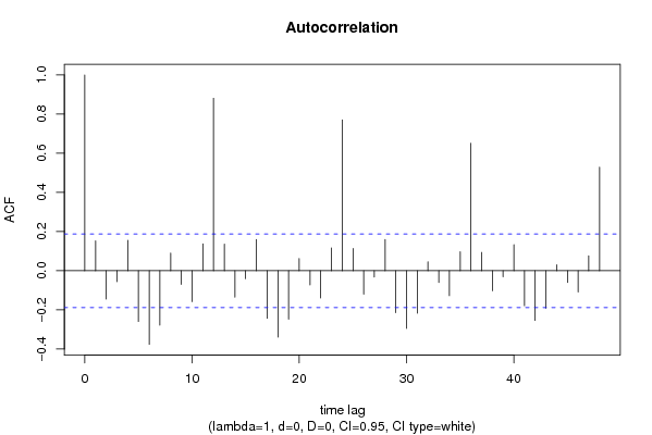
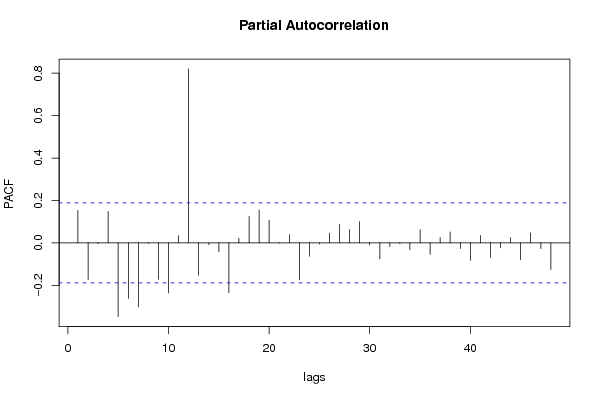
Paste this QR Code to cite your computation.

Original text written by user:

Autocorrelatie van het indexcijfer van de Boekenverkoop in Noorwegen (2001-2009)

IsPrivate?

No (this computation is public)

User-defined keywords

KDGP2W12

Estimated Impact

155

Family? (F = Feedback message, R = changed R code, M = changed R Module, P = changed Parameters, D = changed Data)

-     [Mean Plot] [Boxplot boekenver...] [2010-11-14 19:37:47] [c3c8c498e4d3904156119cc0b4f4389b]
- RMP     [(Partial) Autocorrelation Function] [Autocorrelatie Bo...] [2010-11-17 15:36:10] [d2d436c33b2083ac16b3a67b544ba71f] [Current]

Feedback Forum

Post a new message

Dataseries X:

Download CSV

Histogram

Boxplots

Summary of computational transaction
Raw Input	view raw input (R code)
Raw Output	view raw output of R engine
Computing time	2 seconds
R Server	'RServer@AstonUniversity' @ vre.aston.ac.uk

\begin{tabular}{lllllllll}
\hline
Summary of computational transaction \tabularnewline
Raw Input & view raw input (R code)  \tabularnewline
Raw Output & view raw output of R engine  \tabularnewline
Computing time & 2 seconds \tabularnewline
R Server & 'RServer@AstonUniversity' @ vre.aston.ac.uk \tabularnewline
\hline
\end{tabular}
%Source: https://freestatistics.org/blog/index.php?pk=96732&T=0

[TABLE]
[ROW][C]Summary of computational transaction[/C][/ROW]
[ROW][C]Raw Input[/C][C]view raw input (R code) [/C][/ROW]
[ROW][C]Raw Output[/C][C]view raw output of R engine [/C][/ROW]
[ROW][C]Computing time[/C][C]2 seconds[/C][/ROW]
[ROW][C]R Server[/C][C]'RServer@AstonUniversity' @ vre.aston.ac.uk[/C][/ROW]
[/TABLE]
Source: https://freestatistics.org/blog/index.php?pk=96732&T=0

Globally Unique Identifier (entire table): ba.freestatistics.org/blog/index.php?pk=96732&T=0

As an alternative you can also use a QR Code:

The GUIDs for individual cells are displayed in the table below:

Summary of computational transaction
Raw Input	view raw input (R code)
Raw Output	view raw output of R engine
Computing time	2 seconds
R Server	'RServer@AstonUniversity' @ vre.aston.ac.uk

Autocorrelation Function
Time lag k	ACF(k)	T-STAT	P-value
1	0.152917	1.5892	0.057473
2	-0.145397	-1.511	0.066853
3	-0.055985	-0.5818	0.280954
4	0.154922	1.61	0.055159
5	-0.25948	-2.6966	0.004064
6	-0.376109	-3.9086	8.1e-05
7	-0.278642	-2.8957	0.00229
8	0.090021	0.9355	0.175803
9	-0.070119	-0.7287	0.233881
10	-0.158237	-1.6444	0.051496
11	0.137454	1.4285	0.078022
12	0.881173	9.1574	0
13	0.136216	1.4156	0.079886
14	-0.134658	-1.3994	0.082279
15	-0.040943	-0.4255	0.33566
16	0.159324	1.6557	0.050338
17	-0.2436	-2.5316	0.006397
18	-0.339798	-3.5313	0.000305
19	-0.247527	-2.5724	0.005729
20	0.062311	0.6476	0.259323
21	-0.072924	-0.7579	0.225096
22	-0.139471	-1.4494	0.075058
23	0.116953	1.2154	0.113431
24	0.770941	8.0118	0
25	0.114045	1.1852	0.119271
26	-0.119572	-1.2426	0.108347
27	-0.032705	-0.3399	0.367302
28	0.159554	1.6581	0.050096
29	-0.214073	-2.2247	0.01409
30	-0.294488	-3.0604	0.001394
31	-0.217091	-2.2561	0.01304
32	0.045512	0.473	0.318593
33	-0.059728	-0.6207	0.268049
34	-0.127616	-1.3262	0.093782
35	0.097356	1.0117	0.15696
36	0.651165	6.7671	0
37	0.093487	0.9715	0.166723
38	-0.102479	-1.065	0.144628
39	-0.031102	-0.3232	0.373576
40	0.133308	1.3854	0.084396
41	-0.179005	-1.8603	0.032784
42	-0.253751	-2.6371	0.004798
43	-0.191558	-1.9907	0.024519
44	0.030801	0.3201	0.374758
45	-0.060124	-0.6248	0.266702
46	-0.109285	-1.1357	0.129293
47	0.076662	0.7967	0.213689
48	0.52939	5.5016	0

\begin{tabular}{lllllllll}
\hline
Autocorrelation Function \tabularnewline
Time lag k & ACF(k) & T-STAT & P-value \tabularnewline
1 & 0.152917 & 1.5892 & 0.057473 \tabularnewline
2 & -0.145397 & -1.511 & 0.066853 \tabularnewline
3 & -0.055985 & -0.5818 & 0.280954 \tabularnewline
4 & 0.154922 & 1.61 & 0.055159 \tabularnewline
5 & -0.25948 & -2.6966 & 0.004064 \tabularnewline
6 & -0.376109 & -3.9086 & 8.1e-05 \tabularnewline
7 & -0.278642 & -2.8957 & 0.00229 \tabularnewline
8 & 0.090021 & 0.9355 & 0.175803 \tabularnewline
9 & -0.070119 & -0.7287 & 0.233881 \tabularnewline
10 & -0.158237 & -1.6444 & 0.051496 \tabularnewline
11 & 0.137454 & 1.4285 & 0.078022 \tabularnewline
12 & 0.881173 & 9.1574 & 0 \tabularnewline
13 & 0.136216 & 1.4156 & 0.079886 \tabularnewline
14 & -0.134658 & -1.3994 & 0.082279 \tabularnewline
15 & -0.040943 & -0.4255 & 0.33566 \tabularnewline
16 & 0.159324 & 1.6557 & 0.050338 \tabularnewline
17 & -0.2436 & -2.5316 & 0.006397 \tabularnewline
18 & -0.339798 & -3.5313 & 0.000305 \tabularnewline
19 & -0.247527 & -2.5724 & 0.005729 \tabularnewline
20 & 0.062311 & 0.6476 & 0.259323 \tabularnewline
21 & -0.072924 & -0.7579 & 0.225096 \tabularnewline
22 & -0.139471 & -1.4494 & 0.075058 \tabularnewline
23 & 0.116953 & 1.2154 & 0.113431 \tabularnewline
24 & 0.770941 & 8.0118 & 0 \tabularnewline
25 & 0.114045 & 1.1852 & 0.119271 \tabularnewline
26 & -0.119572 & -1.2426 & 0.108347 \tabularnewline
27 & -0.032705 & -0.3399 & 0.367302 \tabularnewline
28 & 0.159554 & 1.6581 & 0.050096 \tabularnewline
29 & -0.214073 & -2.2247 & 0.01409 \tabularnewline
30 & -0.294488 & -3.0604 & 0.001394 \tabularnewline
31 & -0.217091 & -2.2561 & 0.01304 \tabularnewline
32 & 0.045512 & 0.473 & 0.318593 \tabularnewline
33 & -0.059728 & -0.6207 & 0.268049 \tabularnewline
34 & -0.127616 & -1.3262 & 0.093782 \tabularnewline
35 & 0.097356 & 1.0117 & 0.15696 \tabularnewline
36 & 0.651165 & 6.7671 & 0 \tabularnewline
37 & 0.093487 & 0.9715 & 0.166723 \tabularnewline
38 & -0.102479 & -1.065 & 0.144628 \tabularnewline
39 & -0.031102 & -0.3232 & 0.373576 \tabularnewline
40 & 0.133308 & 1.3854 & 0.084396 \tabularnewline
41 & -0.179005 & -1.8603 & 0.032784 \tabularnewline
42 & -0.253751 & -2.6371 & 0.004798 \tabularnewline
43 & -0.191558 & -1.9907 & 0.024519 \tabularnewline
44 & 0.030801 & 0.3201 & 0.374758 \tabularnewline
45 & -0.060124 & -0.6248 & 0.266702 \tabularnewline
46 & -0.109285 & -1.1357 & 0.129293 \tabularnewline
47 & 0.076662 & 0.7967 & 0.213689 \tabularnewline
48 & 0.52939 & 5.5016 & 0 \tabularnewline
\hline
\end{tabular}
%Source: https://freestatistics.org/blog/index.php?pk=96732&T=1

[TABLE]
[ROW][C]Autocorrelation Function[/C][/ROW]
[ROW][C]Time lag k[/C][C]ACF(k)[/C][C]T-STAT[/C][C]P-value[/C][/ROW]
[ROW][C]1[/C][C]0.152917[/C][C]1.5892[/C][C]0.057473[/C][/ROW]
[ROW][C]2[/C][C]-0.145397[/C][C]-1.511[/C][C]0.066853[/C][/ROW]
[ROW][C]3[/C][C]-0.055985[/C][C]-0.5818[/C][C]0.280954[/C][/ROW]
[ROW][C]4[/C][C]0.154922[/C][C]1.61[/C][C]0.055159[/C][/ROW]
[ROW][C]5[/C][C]-0.25948[/C][C]-2.6966[/C][C]0.004064[/C][/ROW]
[ROW][C]6[/C][C]-0.376109[/C][C]-3.9086[/C][C]8.1e-05[/C][/ROW]
[ROW][C]7[/C][C]-0.278642[/C][C]-2.8957[/C][C]0.00229[/C][/ROW]
[ROW][C]8[/C][C]0.090021[/C][C]0.9355[/C][C]0.175803[/C][/ROW]
[ROW][C]9[/C][C]-0.070119[/C][C]-0.7287[/C][C]0.233881[/C][/ROW]
[ROW][C]10[/C][C]-0.158237[/C][C]-1.6444[/C][C]0.051496[/C][/ROW]
[ROW][C]11[/C][C]0.137454[/C][C]1.4285[/C][C]0.078022[/C][/ROW]
[ROW][C]12[/C][C]0.881173[/C][C]9.1574[/C][C]0[/C][/ROW]
[ROW][C]13[/C][C]0.136216[/C][C]1.4156[/C][C]0.079886[/C][/ROW]
[ROW][C]14[/C][C]-0.134658[/C][C]-1.3994[/C][C]0.082279[/C][/ROW]
[ROW][C]15[/C][C]-0.040943[/C][C]-0.4255[/C][C]0.33566[/C][/ROW]
[ROW][C]16[/C][C]0.159324[/C][C]1.6557[/C][C]0.050338[/C][/ROW]
[ROW][C]17[/C][C]-0.2436[/C][C]-2.5316[/C][C]0.006397[/C][/ROW]
[ROW][C]18[/C][C]-0.339798[/C][C]-3.5313[/C][C]0.000305[/C][/ROW]
[ROW][C]19[/C][C]-0.247527[/C][C]-2.5724[/C][C]0.005729[/C][/ROW]
[ROW][C]20[/C][C]0.062311[/C][C]0.6476[/C][C]0.259323[/C][/ROW]
[ROW][C]21[/C][C]-0.072924[/C][C]-0.7579[/C][C]0.225096[/C][/ROW]
[ROW][C]22[/C][C]-0.139471[/C][C]-1.4494[/C][C]0.075058[/C][/ROW]
[ROW][C]23[/C][C]0.116953[/C][C]1.2154[/C][C]0.113431[/C][/ROW]
[ROW][C]24[/C][C]0.770941[/C][C]8.0118[/C][C]0[/C][/ROW]
[ROW][C]25[/C][C]0.114045[/C][C]1.1852[/C][C]0.119271[/C][/ROW]
[ROW][C]26[/C][C]-0.119572[/C][C]-1.2426[/C][C]0.108347[/C][/ROW]
[ROW][C]27[/C][C]-0.032705[/C][C]-0.3399[/C][C]0.367302[/C][/ROW]
[ROW][C]28[/C][C]0.159554[/C][C]1.6581[/C][C]0.050096[/C][/ROW]
[ROW][C]29[/C][C]-0.214073[/C][C]-2.2247[/C][C]0.01409[/C][/ROW]
[ROW][C]30[/C][C]-0.294488[/C][C]-3.0604[/C][C]0.001394[/C][/ROW]
[ROW][C]31[/C][C]-0.217091[/C][C]-2.2561[/C][C]0.01304[/C][/ROW]
[ROW][C]32[/C][C]0.045512[/C][C]0.473[/C][C]0.318593[/C][/ROW]
[ROW][C]33[/C][C]-0.059728[/C][C]-0.6207[/C][C]0.268049[/C][/ROW]
[ROW][C]34[/C][C]-0.127616[/C][C]-1.3262[/C][C]0.093782[/C][/ROW]
[ROW][C]35[/C][C]0.097356[/C][C]1.0117[/C][C]0.15696[/C][/ROW]
[ROW][C]36[/C][C]0.651165[/C][C]6.7671[/C][C]0[/C][/ROW]
[ROW][C]37[/C][C]0.093487[/C][C]0.9715[/C][C]0.166723[/C][/ROW]
[ROW][C]38[/C][C]-0.102479[/C][C]-1.065[/C][C]0.144628[/C][/ROW]
[ROW][C]39[/C][C]-0.031102[/C][C]-0.3232[/C][C]0.373576[/C][/ROW]
[ROW][C]40[/C][C]0.133308[/C][C]1.3854[/C][C]0.084396[/C][/ROW]
[ROW][C]41[/C][C]-0.179005[/C][C]-1.8603[/C][C]0.032784[/C][/ROW]
[ROW][C]42[/C][C]-0.253751[/C][C]-2.6371[/C][C]0.004798[/C][/ROW]
[ROW][C]43[/C][C]-0.191558[/C][C]-1.9907[/C][C]0.024519[/C][/ROW]
[ROW][C]44[/C][C]0.030801[/C][C]0.3201[/C][C]0.374758[/C][/ROW]
[ROW][C]45[/C][C]-0.060124[/C][C]-0.6248[/C][C]0.266702[/C][/ROW]
[ROW][C]46[/C][C]-0.109285[/C][C]-1.1357[/C][C]0.129293[/C][/ROW]
[ROW][C]47[/C][C]0.076662[/C][C]0.7967[/C][C]0.213689[/C][/ROW]
[ROW][C]48[/C][C]0.52939[/C][C]5.5016[/C][C]0[/C][/ROW]
[/TABLE]
Source: https://freestatistics.org/blog/index.php?pk=96732&T=1

Globally Unique Identifier (entire table): ba.freestatistics.org/blog/index.php?pk=96732&T=1

As an alternative you can also use a QR Code:

The GUIDs for individual cells are displayed in the table below:

Autocorrelation Function
Time lag k	ACF(k)	T-STAT	P-value
1	0.152917	1.5892	0.057473
2	-0.145397	-1.511	0.066853
3	-0.055985	-0.5818	0.280954
4	0.154922	1.61	0.055159
5	-0.25948	-2.6966	0.004064
6	-0.376109	-3.9086	8.1e-05
7	-0.278642	-2.8957	0.00229
8	0.090021	0.9355	0.175803
9	-0.070119	-0.7287	0.233881
10	-0.158237	-1.6444	0.051496
11	0.137454	1.4285	0.078022
12	0.881173	9.1574	0
13	0.136216	1.4156	0.079886
14	-0.134658	-1.3994	0.082279
15	-0.040943	-0.4255	0.33566
16	0.159324	1.6557	0.050338
17	-0.2436	-2.5316	0.006397
18	-0.339798	-3.5313	0.000305
19	-0.247527	-2.5724	0.005729
20	0.062311	0.6476	0.259323
21	-0.072924	-0.7579	0.225096
22	-0.139471	-1.4494	0.075058
23	0.116953	1.2154	0.113431
24	0.770941	8.0118	0
25	0.114045	1.1852	0.119271
26	-0.119572	-1.2426	0.108347
27	-0.032705	-0.3399	0.367302
28	0.159554	1.6581	0.050096
29	-0.214073	-2.2247	0.01409
30	-0.294488	-3.0604	0.001394
31	-0.217091	-2.2561	0.01304
32	0.045512	0.473	0.318593
33	-0.059728	-0.6207	0.268049
34	-0.127616	-1.3262	0.093782
35	0.097356	1.0117	0.15696
36	0.651165	6.7671	0
37	0.093487	0.9715	0.166723
38	-0.102479	-1.065	0.144628
39	-0.031102	-0.3232	0.373576
40	0.133308	1.3854	0.084396
41	-0.179005	-1.8603	0.032784
42	-0.253751	-2.6371	0.004798
43	-0.191558	-1.9907	0.024519
44	0.030801	0.3201	0.374758
45	-0.060124	-0.6248	0.266702
46	-0.109285	-1.1357	0.129293
47	0.076662	0.7967	0.213689
48	0.52939	5.5016	0

Partial Autocorrelation Function
Time lag k	PACF(k)	T-STAT	P-value
1	0.152917	1.5892	0.057473
2	-0.172822	-1.796	0.037643
3	-0.003674	-0.0382	0.484808
4	0.148249	1.5407	0.063163
5	-0.348059	-3.6171	0.000227
6	-0.261014	-2.7125	0.003886
7	-0.301847	-3.1369	0.0011
8	-0.003307	-0.0344	0.486323
9	-0.171372	-1.7809	0.038866
10	-0.236311	-2.4558	0.007826
11	0.034329	0.3568	0.360984
12	0.820176	8.5235	0
13	-0.153371	-1.5939	0.056943
14	-0.008612	-0.0895	0.464427
15	-0.042025	-0.4367	0.331587
16	-0.235581	-2.4482	0.007983
17	0.021273	0.2211	0.412724
18	0.12411	1.2898	0.099939
19	0.154775	1.6085	0.055326
20	0.106643	1.1083	0.135103
21	-0.00143	-0.0149	0.494085
22	0.037966	0.3946	0.346975
23	-0.173893	-1.8071	0.036762
24	-0.062697	-0.6516	0.258032
25	-0.005825	-0.0605	0.475919
26	0.045444	0.4723	0.318844
27	0.086468	0.8986	0.185433
28	0.063433	0.6592	0.25558
29	0.099684	1.036	0.15127
30	-0.010006	-0.104	0.458688
31	-0.074939	-0.7788	0.218905
32	-0.017232	-0.1791	0.429106
33	-0.003196	-0.0332	0.486784
34	-0.031563	-0.328	0.37177
35	0.061789	0.6421	0.261073
36	-0.054247	-0.5638	0.287045
37	0.025371	0.2637	0.396272
38	0.051648	0.5367	0.296276
39	-0.0265	-0.2754	0.391769
40	-0.082209	-0.8543	0.197404
41	0.034737	0.361	0.359403
42	-0.067716	-0.7037	0.241558
43	-0.023407	-0.2432	0.404137
44	0.023895	0.2483	0.402176
45	-0.080183	-0.8333	0.203261
46	0.046678	0.4851	0.314297
47	-0.0265	-0.2754	0.391768
48	-0.125165	-1.3008	0.098056

\begin{tabular}{lllllllll}
\hline
Partial Autocorrelation Function \tabularnewline
Time lag k & PACF(k) & T-STAT & P-value \tabularnewline
1 & 0.152917 & 1.5892 & 0.057473 \tabularnewline
2 & -0.172822 & -1.796 & 0.037643 \tabularnewline
3 & -0.003674 & -0.0382 & 0.484808 \tabularnewline
4 & 0.148249 & 1.5407 & 0.063163 \tabularnewline
5 & -0.348059 & -3.6171 & 0.000227 \tabularnewline
6 & -0.261014 & -2.7125 & 0.003886 \tabularnewline
7 & -0.301847 & -3.1369 & 0.0011 \tabularnewline
8 & -0.003307 & -0.0344 & 0.486323 \tabularnewline
9 & -0.171372 & -1.7809 & 0.038866 \tabularnewline
10 & -0.236311 & -2.4558 & 0.007826 \tabularnewline
11 & 0.034329 & 0.3568 & 0.360984 \tabularnewline
12 & 0.820176 & 8.5235 & 0 \tabularnewline
13 & -0.153371 & -1.5939 & 0.056943 \tabularnewline
14 & -0.008612 & -0.0895 & 0.464427 \tabularnewline
15 & -0.042025 & -0.4367 & 0.331587 \tabularnewline
16 & -0.235581 & -2.4482 & 0.007983 \tabularnewline
17 & 0.021273 & 0.2211 & 0.412724 \tabularnewline
18 & 0.12411 & 1.2898 & 0.099939 \tabularnewline
19 & 0.154775 & 1.6085 & 0.055326 \tabularnewline
20 & 0.106643 & 1.1083 & 0.135103 \tabularnewline
21 & -0.00143 & -0.0149 & 0.494085 \tabularnewline
22 & 0.037966 & 0.3946 & 0.346975 \tabularnewline
23 & -0.173893 & -1.8071 & 0.036762 \tabularnewline
24 & -0.062697 & -0.6516 & 0.258032 \tabularnewline
25 & -0.005825 & -0.0605 & 0.475919 \tabularnewline
26 & 0.045444 & 0.4723 & 0.318844 \tabularnewline
27 & 0.086468 & 0.8986 & 0.185433 \tabularnewline
28 & 0.063433 & 0.6592 & 0.25558 \tabularnewline
29 & 0.099684 & 1.036 & 0.15127 \tabularnewline
30 & -0.010006 & -0.104 & 0.458688 \tabularnewline
31 & -0.074939 & -0.7788 & 0.218905 \tabularnewline
32 & -0.017232 & -0.1791 & 0.429106 \tabularnewline
33 & -0.003196 & -0.0332 & 0.486784 \tabularnewline
34 & -0.031563 & -0.328 & 0.37177 \tabularnewline
35 & 0.061789 & 0.6421 & 0.261073 \tabularnewline
36 & -0.054247 & -0.5638 & 0.287045 \tabularnewline
37 & 0.025371 & 0.2637 & 0.396272 \tabularnewline
38 & 0.051648 & 0.5367 & 0.296276 \tabularnewline
39 & -0.0265 & -0.2754 & 0.391769 \tabularnewline
40 & -0.082209 & -0.8543 & 0.197404 \tabularnewline
41 & 0.034737 & 0.361 & 0.359403 \tabularnewline
42 & -0.067716 & -0.7037 & 0.241558 \tabularnewline
43 & -0.023407 & -0.2432 & 0.404137 \tabularnewline
44 & 0.023895 & 0.2483 & 0.402176 \tabularnewline
45 & -0.080183 & -0.8333 & 0.203261 \tabularnewline
46 & 0.046678 & 0.4851 & 0.314297 \tabularnewline
47 & -0.0265 & -0.2754 & 0.391768 \tabularnewline
48 & -0.125165 & -1.3008 & 0.098056 \tabularnewline
\hline
\end{tabular}
%Source: https://freestatistics.org/blog/index.php?pk=96732&T=2

[TABLE]
[ROW][C]Partial Autocorrelation Function[/C][/ROW]
[ROW][C]Time lag k[/C][C]PACF(k)[/C][C]T-STAT[/C][C]P-value[/C][/ROW]
[ROW][C]1[/C][C]0.152917[/C][C]1.5892[/C][C]0.057473[/C][/ROW]
[ROW][C]2[/C][C]-0.172822[/C][C]-1.796[/C][C]0.037643[/C][/ROW]
[ROW][C]3[/C][C]-0.003674[/C][C]-0.0382[/C][C]0.484808[/C][/ROW]
[ROW][C]4[/C][C]0.148249[/C][C]1.5407[/C][C]0.063163[/C][/ROW]
[ROW][C]5[/C][C]-0.348059[/C][C]-3.6171[/C][C]0.000227[/C][/ROW]
[ROW][C]6[/C][C]-0.261014[/C][C]-2.7125[/C][C]0.003886[/C][/ROW]
[ROW][C]7[/C][C]-0.301847[/C][C]-3.1369[/C][C]0.0011[/C][/ROW]
[ROW][C]8[/C][C]-0.003307[/C][C]-0.0344[/C][C]0.486323[/C][/ROW]
[ROW][C]9[/C][C]-0.171372[/C][C]-1.7809[/C][C]0.038866[/C][/ROW]
[ROW][C]10[/C][C]-0.236311[/C][C]-2.4558[/C][C]0.007826[/C][/ROW]
[ROW][C]11[/C][C]0.034329[/C][C]0.3568[/C][C]0.360984[/C][/ROW]
[ROW][C]12[/C][C]0.820176[/C][C]8.5235[/C][C]0[/C][/ROW]
[ROW][C]13[/C][C]-0.153371[/C][C]-1.5939[/C][C]0.056943[/C][/ROW]
[ROW][C]14[/C][C]-0.008612[/C][C]-0.0895[/C][C]0.464427[/C][/ROW]
[ROW][C]15[/C][C]-0.042025[/C][C]-0.4367[/C][C]0.331587[/C][/ROW]
[ROW][C]16[/C][C]-0.235581[/C][C]-2.4482[/C][C]0.007983[/C][/ROW]
[ROW][C]17[/C][C]0.021273[/C][C]0.2211[/C][C]0.412724[/C][/ROW]
[ROW][C]18[/C][C]0.12411[/C][C]1.2898[/C][C]0.099939[/C][/ROW]
[ROW][C]19[/C][C]0.154775[/C][C]1.6085[/C][C]0.055326[/C][/ROW]
[ROW][C]20[/C][C]0.106643[/C][C]1.1083[/C][C]0.135103[/C][/ROW]
[ROW][C]21[/C][C]-0.00143[/C][C]-0.0149[/C][C]0.494085[/C][/ROW]
[ROW][C]22[/C][C]0.037966[/C][C]0.3946[/C][C]0.346975[/C][/ROW]
[ROW][C]23[/C][C]-0.173893[/C][C]-1.8071[/C][C]0.036762[/C][/ROW]
[ROW][C]24[/C][C]-0.062697[/C][C]-0.6516[/C][C]0.258032[/C][/ROW]
[ROW][C]25[/C][C]-0.005825[/C][C]-0.0605[/C][C]0.475919[/C][/ROW]
[ROW][C]26[/C][C]0.045444[/C][C]0.4723[/C][C]0.318844[/C][/ROW]
[ROW][C]27[/C][C]0.086468[/C][C]0.8986[/C][C]0.185433[/C][/ROW]
[ROW][C]28[/C][C]0.063433[/C][C]0.6592[/C][C]0.25558[/C][/ROW]
[ROW][C]29[/C][C]0.099684[/C][C]1.036[/C][C]0.15127[/C][/ROW]
[ROW][C]30[/C][C]-0.010006[/C][C]-0.104[/C][C]0.458688[/C][/ROW]
[ROW][C]31[/C][C]-0.074939[/C][C]-0.7788[/C][C]0.218905[/C][/ROW]
[ROW][C]32[/C][C]-0.017232[/C][C]-0.1791[/C][C]0.429106[/C][/ROW]
[ROW][C]33[/C][C]-0.003196[/C][C]-0.0332[/C][C]0.486784[/C][/ROW]
[ROW][C]34[/C][C]-0.031563[/C][C]-0.328[/C][C]0.37177[/C][/ROW]
[ROW][C]35[/C][C]0.061789[/C][C]0.6421[/C][C]0.261073[/C][/ROW]
[ROW][C]36[/C][C]-0.054247[/C][C]-0.5638[/C][C]0.287045[/C][/ROW]
[ROW][C]37[/C][C]0.025371[/C][C]0.2637[/C][C]0.396272[/C][/ROW]
[ROW][C]38[/C][C]0.051648[/C][C]0.5367[/C][C]0.296276[/C][/ROW]
[ROW][C]39[/C][C]-0.0265[/C][C]-0.2754[/C][C]0.391769[/C][/ROW]
[ROW][C]40[/C][C]-0.082209[/C][C]-0.8543[/C][C]0.197404[/C][/ROW]
[ROW][C]41[/C][C]0.034737[/C][C]0.361[/C][C]0.359403[/C][/ROW]
[ROW][C]42[/C][C]-0.067716[/C][C]-0.7037[/C][C]0.241558[/C][/ROW]
[ROW][C]43[/C][C]-0.023407[/C][C]-0.2432[/C][C]0.404137[/C][/ROW]
[ROW][C]44[/C][C]0.023895[/C][C]0.2483[/C][C]0.402176[/C][/ROW]
[ROW][C]45[/C][C]-0.080183[/C][C]-0.8333[/C][C]0.203261[/C][/ROW]
[ROW][C]46[/C][C]0.046678[/C][C]0.4851[/C][C]0.314297[/C][/ROW]
[ROW][C]47[/C][C]-0.0265[/C][C]-0.2754[/C][C]0.391768[/C][/ROW]
[ROW][C]48[/C][C]-0.125165[/C][C]-1.3008[/C][C]0.098056[/C][/ROW]
[/TABLE]
Source: https://freestatistics.org/blog/index.php?pk=96732&T=2

Globally Unique Identifier (entire table): ba.freestatistics.org/blog/index.php?pk=96732&T=2

As an alternative you can also use a QR Code:

The GUIDs for individual cells are displayed in the table below:

Partial Autocorrelation Function
Time lag k	PACF(k)	T-STAT	P-value
1	0.152917	1.5892	0.057473
2	-0.172822	-1.796	0.037643
3	-0.003674	-0.0382	0.484808
4	0.148249	1.5407	0.063163
5	-0.348059	-3.6171	0.000227
6	-0.261014	-2.7125	0.003886
7	-0.301847	-3.1369	0.0011
8	-0.003307	-0.0344	0.486323
9	-0.171372	-1.7809	0.038866
10	-0.236311	-2.4558	0.007826
11	0.034329	0.3568	0.360984
12	0.820176	8.5235	0
13	-0.153371	-1.5939	0.056943
14	-0.008612	-0.0895	0.464427
15	-0.042025	-0.4367	0.331587
16	-0.235581	-2.4482	0.007983
17	0.021273	0.2211	0.412724
18	0.12411	1.2898	0.099939
19	0.154775	1.6085	0.055326
20	0.106643	1.1083	0.135103
21	-0.00143	-0.0149	0.494085
22	0.037966	0.3946	0.346975
23	-0.173893	-1.8071	0.036762
24	-0.062697	-0.6516	0.258032
25	-0.005825	-0.0605	0.475919
26	0.045444	0.4723	0.318844
27	0.086468	0.8986	0.185433
28	0.063433	0.6592	0.25558
29	0.099684	1.036	0.15127
30	-0.010006	-0.104	0.458688
31	-0.074939	-0.7788	0.218905
32	-0.017232	-0.1791	0.429106
33	-0.003196	-0.0332	0.486784
34	-0.031563	-0.328	0.37177
35	0.061789	0.6421	0.261073
36	-0.054247	-0.5638	0.287045
37	0.025371	0.2637	0.396272
38	0.051648	0.5367	0.296276
39	-0.0265	-0.2754	0.391769
40	-0.082209	-0.8543	0.197404
41	0.034737	0.361	0.359403
42	-0.067716	-0.7037	0.241558
43	-0.023407	-0.2432	0.404137
44	0.023895	0.2483	0.402176
45	-0.080183	-0.8333	0.203261
46	0.046678	0.4851	0.314297
47	-0.0265	-0.2754	0.391768
48	-0.125165	-1.3008	0.098056

Figure 1

PNG link

Postscript link

PDF link

Figure 2

PNG link

Postscript link

PDF link

Parameters (Session):

par1 = 48 ; par2 = 1 ; par3 = 0 ; par4 = 0 ; par5 = 12 ; par6 = White Noise ; par7 = 0.95 ;

Parameters (R input):

par1 = 48 ; par2 = 1 ; par3 = 0 ; par4 = 0 ; par5 = 12 ; par6 = White Noise ; par7 = 0.95 ;

R code (references can be found in the software module):

if (par1 == 'Default') {
par1 = 10*log10(length(x))
} else {
par1 <- as.numeric(par1)
}
par2 <- as.numeric(par2)
par3 <- as.numeric(par3)
par4 <- as.numeric(par4)
par5 <- as.numeric(par5)
if (par6 == 'White Noise') par6 <- 'white' else par6 <- 'ma'
par7 <- as.numeric(par7)
if (par2 == 0) {
x <- log(x)
} else {
x <- (x ^ par2 - 1) / par2
}
if (par3 > 0) x <- diff(x,lag=1,difference=par3)
if (par4 > 0) x <- diff(x,lag=par5,difference=par4)
bitmap(file='pic1.png')
racf <- acf(x, par1, main='Autocorrelation', xlab='time lag', ylab='ACF', ci.type=par6, ci=par7, sub=paste('(lambda=',par2,', d=',par3,', D=',par4,', CI=', par7, ', CI type=',par6,')',sep=''))
dev.off()
bitmap(file='pic2.png')
rpacf <- pacf(x,par1,main='Partial Autocorrelation',xlab='lags',ylab='PACF')
dev.off()
(myacf <- c(racf$acf))
(mypacf <- c(rpacf$acf))
lengthx <- length(x)
sqrtn <- sqrt(lengthx)
load(file='createtable')
a<-table.start()
a<-table.row.start(a)
a<-table.element(a,'Autocorrelation Function',4,TRUE)
a<-table.row.end(a)
a<-table.row.start(a)
a<-table.element(a,'Time lag k',header=TRUE)
a<-table.element(a,hyperlink('basics.htm','ACF(k)','click here for more information about the Autocorrelation Function'),header=TRUE)
a<-table.element(a,'T-STAT',header=TRUE)
a<-table.element(a,'P-value',header=TRUE)
a<-table.row.end(a)
for (i in 2:(par1+1)) {
a<-table.row.start(a)
a<-table.element(a,i-1,header=TRUE)
a<-table.element(a,round(myacf[i],6))
mytstat <- myacf[i]*sqrtn
a<-table.element(a,round(mytstat,4))
a<-table.element(a,round(1-pt(abs(mytstat),lengthx),6))
a<-table.row.end(a)
}
a<-table.end(a)
table.save(a,file='mytable.tab')
a<-table.start()
a<-table.row.start(a)
a<-table.element(a,'Partial Autocorrelation Function',4,TRUE)
a<-table.row.end(a)
a<-table.row.start(a)
a<-table.element(a,'Time lag k',header=TRUE)
a<-table.element(a,hyperlink('basics.htm','PACF(k)','click here for more information about the Partial Autocorrelation Function'),header=TRUE)
a<-table.element(a,'T-STAT',header=TRUE)
a<-table.element(a,'P-value',header=TRUE)
a<-table.row.end(a)
for (i in 1:par1) {
a<-table.row.start(a)
a<-table.element(a,i,header=TRUE)
a<-table.element(a,round(mypacf[i],6))
mytstat <- mypacf[i]*sqrtn
a<-table.element(a,round(mytstat,4))
a<-table.element(a,round(1-pt(abs(mytstat),lengthx),6))
a<-table.row.end(a)
}
a<-table.end(a)
table.save(a,file='mytable1.tab')

Free Statistics

Description of Statistical Computation

Tree of Dependent Computations

Dataset

Tables (Output of Computation)

Figures (Output of Computation)

Input Parameters & R Code