Free Statistics
of Irreproducible Research!
Description of Statistical Computation | |||||||||||||||||||||
|---|---|---|---|---|---|---|---|---|---|---|---|---|---|---|---|---|---|---|---|---|---|
| Author's title | |||||||||||||||||||||
| Author | *Unverified author* | ||||||||||||||||||||
| R Software Module | rwasp_meanplot.wasp | ||||||||||||||||||||
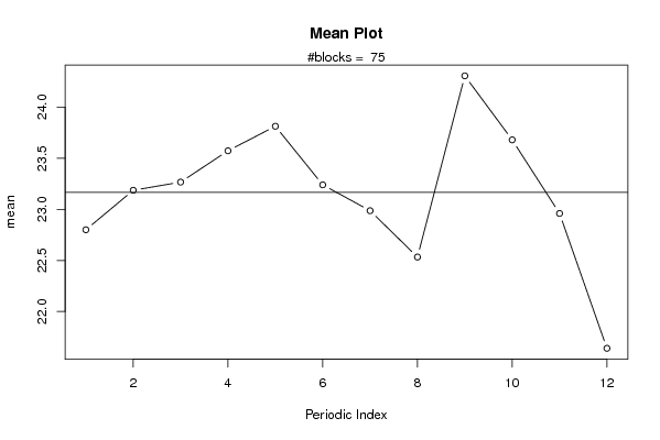
| Title produced by software | Mean Plot | ||||||||||||||||||||
| Date of computation | Wed, 17 Nov 2010 09:45:10 +0000 | ||||||||||||||||||||
| Cite this page as follows | Statistical Computations at FreeStatistics.org, Office for Research Development and Education, URL https://freestatistics.org/blog/index.php?v=date/2010/Nov/17/t12899870463vt1ywtu8wkp4cg.htm/, Retrieved Thu, 25 Apr 2024 09:10:25 +0000 | ||||||||||||||||||||
| Statistical Computations at FreeStatistics.org, Office for Research Development and Education, URL https://freestatistics.org/blog/index.php?pk=96561, Retrieved Thu, 25 Apr 2024 09:10:25 +0000 | |||||||||||||||||||||
| QR Codes: | |||||||||||||||||||||
|
| |||||||||||||||||||||
| Original text written by user: | |||||||||||||||||||||
| IsPrivate? | No (this computation is public) | ||||||||||||||||||||
| User-defined keywords | KDGP1W52 | ||||||||||||||||||||
| Estimated Impact | 122 | ||||||||||||||||||||
Tree of Dependent Computations | |||||||||||||||||||||
| Family? (F = Feedback message, R = changed R code, M = changed R Module, P = changed Parameters, D = changed Data) | |||||||||||||||||||||
| - [Mean Plot] [] [2010-11-17 09:45:10] [b831d618c4f08b1797d6e909807842bd] [Current] | |||||||||||||||||||||
| Feedback Forum | |||||||||||||||||||||
Post a new message | |||||||||||||||||||||
Dataset | |||||||||||||||||||||
| Dataseries X: | |||||||||||||||||||||
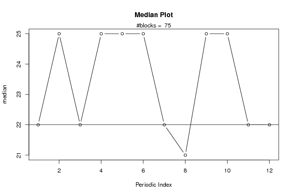
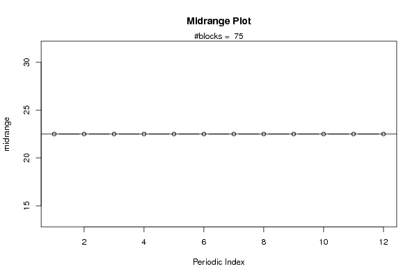
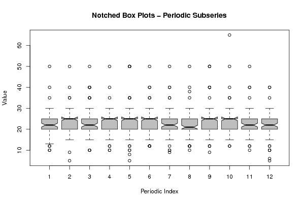
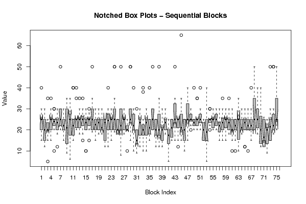
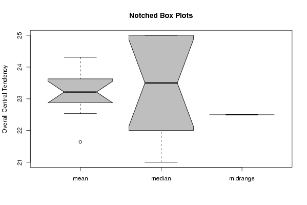
20 25 15 15 25 25 25 21 30 25 20 40 13 30 25 20 25 20 25 20 20 15 15 12 20 5 20 15 25 22 20 22 25 20 20 35 30 25 20 20 20 25 25 15 20 35 25 25 30 23 10 22 25 25 22 30 20 25 25 22 25 25 25 22 25 12 18 20 20 22 30 25 22 20 50 30 25 20 30 22 25 30 22 25 22 22 25 25 25 20 22 15 20 30 20 25 30 35 22 12 30 15 10 30 9 25 20 20 35 25 35 30 12 25 15 25 25 20 20 6 15 40 20 40 25 25 20 15 15 22 24 22 20 25 25 25 35 40 20 22 22 20 25 25 18 25 20 25 30 20 22 35 22 25 25 25 25 22 23 35 15 25 18 22 25 25 28 30 20 25 25 30 22 30 10 10 25 20 22 25 25 15 22 25 25 28 22 30 25 20 25 25 20 30 20 30 50 19 20 28 20 25 35 25 25 15 16 20 20 25 30 20 25 25 25 20 20 25 25 30 22 20 25 25 18 18 20 25 25 30 25 20 25 20 20 20 22 18 22 20 15 25 25 20 25 15 22 25 25 15 12 25 30 22 15 22 25 12 18 30 25 25 40 24 25 15 25 20 25 25 25 20 30 20 25 30 22 25 25 25 50 19 50 25 35 20 20 20 20 20 25 25 25 20 20 20 20 25 18 25 22 22 30 30 8 20 25 30 50 22 20 10 25 25 25 25 18 25 20 25 30 18 20 25 22 22 20 20 25 20 20 20 20 25 20 10 20 25 30 25 50 30 30 50 15 25 25 22 20 22 30 25 18 22 22 30 40 25 20 10 20 9 15 20 15 20 30 12 15 12 20 15 12 25 20 25 25 25 30 20 25 15 15 22 10 15 10 20 25 20 20 38 20 20 20 40 25 25 30 25 10 20 25 12 15 25 20 22 22 20 25 25 25 15 40 20 20 16 25 15 20 25 20 30 50 20 25 20 30 30 25 25 12 25 25 25 20 20 20 15 20 25 15 25 50 30 20 20 25 12 15 20 20 35 22 15 18 30 22 12 12 20 20 15 25 15 20 20 25 18 30 20 25 25 25 20 20 25 20 22 15 15 22 20 10 25 20 20 15 12 20 5 20 15 15 25 25 25 15 25 22 25 20 18 22 25 35 25 25 25 35 30 22 30 50 15 25 24 20 25 25 25 12 15 22 25 25 25 25 15 20 20 15 35 30 20 22 65 20 25 22 20 25 25 20 25 15 20 12 15 10 25 15 30 35 25 25 25 25 25 40 40 25 25 20 25 25 22 25 30 25 25 30 25 25 30 25 25 20 22 22 20 25 22 25 22 40 25 25 25 22 20 35 20 35 25 22 25 25 25 25 25 40 25 30 25 20 25 25 30 22 22 20 15 15 25 25 20 20 15 25 15 20 22 25 15 15 18 5 15 25 18 40 25 25 20 30 20 25 25 25 22 22 25 25 30 25 25 25 25 20 20 25 25 25 25 20 30 25 22 30 20 20 30 25 25 30 20 25 25 24 25 30 18 15 22 22 25 22 22 25 15 20 22 18 35 20 20 20 25 25 30 15 25 22 26 25 20 25 25 25 22 25 25 20 22 30 15 30 25 20 25 25 35 22 20 25 20 20 18 20 22 25 10 20 25 20 20 30 25 20 15 20 25 10 20 25 22 22 25 25 15 25 20 10 25 16 25 35 25 15 25 25 30 25 10 22 20 25 20 20 25 22 18 30 19 25 20 25 20 25 20 22 12 30 12 22 25 25 25 25 30 30 10 22 22 25 20 22 20 25 20 15 25 20 25 20 30 15 40 25 20 22 22 30 20 40 20 25 20 25 20 50 50 25 25 40 30 22 30 20 25 25 30 25 25 20 18 18 28 25 22 15 40 40 12 12 18 12 25 26 18 25 22 15 25 15 15 15 25 15 12 22 20 20 25 20 12 9 15 12 15 25 20 20 15 15 30 21 25 22 22 50 15 25 15 25 22 18 50 20 50 20 20 30 25 20 22 25 50 40 25 25 25 25 30 40 25 30 20 | |||||||||||||||||||||
Tables (Output of Computation) | |||||||||||||||||||||
| |||||||||||||||||||||
Figures (Output of Computation) | |||||||||||||||||||||
Input Parameters & R Code | |||||||||||||||||||||
| Parameters (Session): | |||||||||||||||||||||
| par1 = 12 ; | |||||||||||||||||||||
| Parameters (R input): | |||||||||||||||||||||
| par1 = 12 ; | |||||||||||||||||||||
| R code (references can be found in the software module): | |||||||||||||||||||||
par1 <- as.numeric(par1) | |||||||||||||||||||||