Free Statistics
of Irreproducible Research!
Description of Statistical Computation | |||||||||||||||||||||
|---|---|---|---|---|---|---|---|---|---|---|---|---|---|---|---|---|---|---|---|---|---|
| Author's title | |||||||||||||||||||||
| Author | *Unverified author* | ||||||||||||||||||||
| R Software Module | rwasp_meanplot.wasp | ||||||||||||||||||||
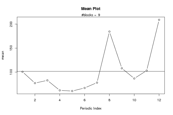
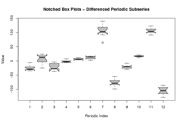
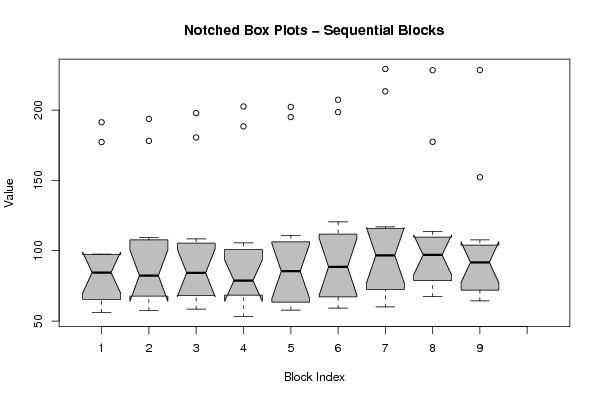
| Title produced by software | Mean Plot | ||||||||||||||||||||
| Date of computation | Sun, 14 Nov 2010 19:37:47 +0000 | ||||||||||||||||||||
| Cite this page as follows | Statistical Computations at FreeStatistics.org, Office for Research Development and Education, URL https://freestatistics.org/blog/index.php?v=date/2010/Nov/14/t12897635121d96ttvyq48owt7.htm/, Retrieved Wed, 24 Apr 2024 13:10:52 +0000 | ||||||||||||||||||||
| Statistical Computations at FreeStatistics.org, Office for Research Development and Education, URL https://freestatistics.org/blog/index.php?pk=94621, Retrieved Wed, 24 Apr 2024 13:10:52 +0000 | |||||||||||||||||||||
| QR Codes: | |||||||||||||||||||||
|
| |||||||||||||||||||||
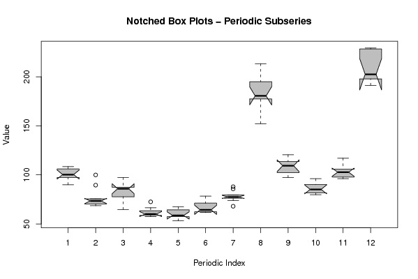
| Original text written by user: | Boxplot van de indexcijfers van de maandelijkse boekenverkoop in Noorwegen van 2001 tot 2009. | ||||||||||||||||||||
| IsPrivate? | No (this computation is public) | ||||||||||||||||||||
| User-defined keywords | KDGP1W52 | ||||||||||||||||||||
| Estimated Impact | 151 | ||||||||||||||||||||
Tree of Dependent Computations | |||||||||||||||||||||
| Family? (F = Feedback message, R = changed R code, M = changed R Module, P = changed Parameters, D = changed Data) | |||||||||||||||||||||
| - [Mean Plot] [Boxplot boekenver...] [2010-11-14 19:37:47] [d2d436c33b2083ac16b3a67b544ba71f] [Current] - RMP [(Partial) Autocorrelation Function] [Autocorrelatie Bo...] [2010-11-17 15:36:10] [c3c8c498e4d3904156119cc0b4f4389b] - RMP [(Partial) Autocorrelation Function] [Autocorrelatie no...] [2010-11-17 15:43:32] [c3c8c498e4d3904156119cc0b4f4389b] | |||||||||||||||||||||
| Feedback Forum | |||||||||||||||||||||
Post a new message | |||||||||||||||||||||
Dataset | |||||||||||||||||||||
| Dataseries X: | |||||||||||||||||||||
90 69,3 87,3 57,4 56,2 61,6 77,7 177,2 97,6 81,6 96,8 191,3 106 75,1 72 63,5 57,4 62,3 79,4 178,1 109,3 85,2 102,7 193,7 108,4 73,4 85,9 58,5 58,6 62,7 77,5 180,5 102,2 82,6 97,8 197,8 93,8 72,4 77,7 58,7 53,1 64,3 76,4 188,4 105,5 79,8 96,1 202,5 97,3 89,5 64,7 61,2 57,8 62 76,3 195 110,9 81,4 101,7 202,2 97,4 68,5 86,8 59,1 62,4 66,2 68 198,5 120,4 90,2 103,2 207,3 106,4 75,5 97,3 60 67,5 71,2 73,7 213,3 114,6 96,1 117 229,2 105,6 99,9 79,3 72,5 67,4 78,3 85,7 177,4 113,6 94,1 105,7 228,3 100,3 70,3 94,2 66,5 64,4 73,7 87,9 152,2 97,3 89,3 107,6 228,4 | |||||||||||||||||||||
Tables (Output of Computation) | |||||||||||||||||||||
| |||||||||||||||||||||
Figures (Output of Computation) | |||||||||||||||||||||
Input Parameters & R Code | |||||||||||||||||||||
| Parameters (Session): | |||||||||||||||||||||
| par1 = 12 ; | |||||||||||||||||||||
| Parameters (R input): | |||||||||||||||||||||
| par1 = 12 ; | |||||||||||||||||||||
| R code (references can be found in the software module): | |||||||||||||||||||||
par1 <- as.numeric(par1) | |||||||||||||||||||||