Free Statistics
of Irreproducible Research!
Description of Statistical Computation | |||||||||||||||||||||
|---|---|---|---|---|---|---|---|---|---|---|---|---|---|---|---|---|---|---|---|---|---|
| Author's title | |||||||||||||||||||||
| Author | *Unverified author* | ||||||||||||||||||||
| R Software Module | rwasp_meanplot.wasp | ||||||||||||||||||||
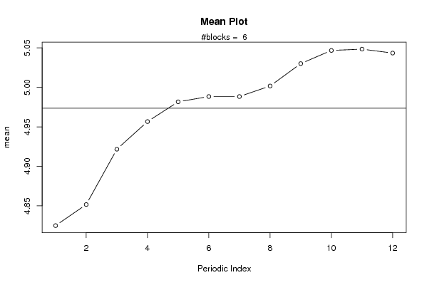
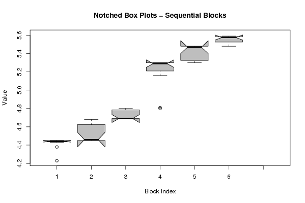
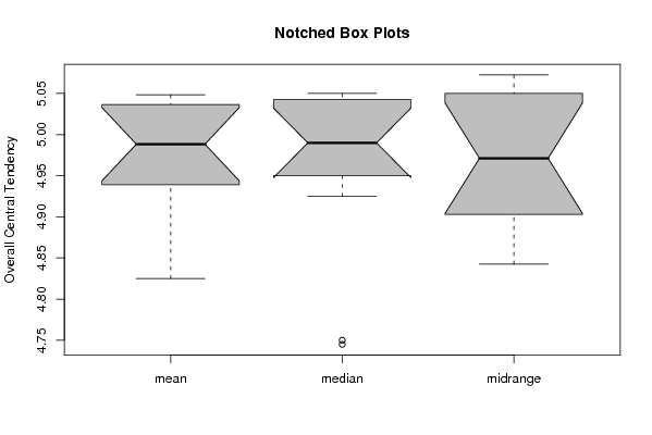
| Title produced by software | Mean Plot | ||||||||||||||||||||
| Date of computation | Sun, 14 Nov 2010 19:13:30 +0000 | ||||||||||||||||||||
| Cite this page as follows | Statistical Computations at FreeStatistics.org, Office for Research Development and Education, URL https://freestatistics.org/blog/index.php?v=date/2010/Nov/14/t128976192698g41sltvia5jis.htm/, Retrieved Sat, 05 Jul 2025 18:55:35 +0000 | ||||||||||||||||||||
| Statistical Computations at FreeStatistics.org, Office for Research Development and Education, URL https://freestatistics.org/blog/index.php?pk=94613, Retrieved Sat, 05 Jul 2025 18:55:35 +0000 | |||||||||||||||||||||
| QR Codes: | |||||||||||||||||||||
|
| |||||||||||||||||||||
| Original text written by user: | |||||||||||||||||||||
| IsPrivate? | No (this computation is public) | ||||||||||||||||||||
| User-defined keywords | KDGP1W52 | ||||||||||||||||||||
| Estimated Impact | 246 | ||||||||||||||||||||
Tree of Dependent Computations | |||||||||||||||||||||
| Family? (F = Feedback message, R = changed R code, M = changed R Module, P = changed Parameters, D = changed Data) | |||||||||||||||||||||
| - [Mean Plot] [Evolutie prijzen ...] [2010-11-14 19:13:30] [384a4ac05535402cc728b569fb124a5f] [Current] | |||||||||||||||||||||
| Feedback Forum | |||||||||||||||||||||
Post a new message | |||||||||||||||||||||
Dataset | |||||||||||||||||||||
| Dataseries X: | |||||||||||||||||||||
4,23 4,38 4,43 4,44 4,44 4,44 4,44 4,44 4,45 4,45 4,45 4,45 4,45 4,45 4,45 4,45 4,46 4,46 4,46 4,48 4,58 4,67 4,68 4,68 4,69 4,69 4,69 4,69 4,69 4,69 4,69 4,73 4,78 4,79 4,79 4,8 4,8 4,81 5,16 5,26 5,29 5,29 5,29 5,3 5,3 5,3 5,3 5,3 5,3 5,3 5,3 5,35 5,44 5,47 5,47 5,48 5,48 5,48 5,48 5,48 5,48 5,48 5,5 5,55 5,57 5,58 5,58 5,58 5,59 5,59 5,59 5,55 | |||||||||||||||||||||
Tables (Output of Computation) | |||||||||||||||||||||
| |||||||||||||||||||||
Figures (Output of Computation) | |||||||||||||||||||||
Input Parameters & R Code | |||||||||||||||||||||
| Parameters (Session): | |||||||||||||||||||||
| par1 = 12 ; | |||||||||||||||||||||
| Parameters (R input): | |||||||||||||||||||||
| par1 = 12 ; | |||||||||||||||||||||
| R code (references can be found in the software module): | |||||||||||||||||||||
par1 <- as.numeric(par1) | |||||||||||||||||||||