Free Statistics
of Irreproducible Research!
Description of Statistical Computation | |||||||||||||||||||||||||||||||||||||||||||||||||||||||||||||
|---|---|---|---|---|---|---|---|---|---|---|---|---|---|---|---|---|---|---|---|---|---|---|---|---|---|---|---|---|---|---|---|---|---|---|---|---|---|---|---|---|---|---|---|---|---|---|---|---|---|---|---|---|---|---|---|---|---|---|---|---|---|
| Author's title | |||||||||||||||||||||||||||||||||||||||||||||||||||||||||||||
| Author | *The author of this computation has been verified* | ||||||||||||||||||||||||||||||||||||||||||||||||||||||||||||
| R Software Module | rwasp_linear_regression.wasp | ||||||||||||||||||||||||||||||||||||||||||||||||||||||||||||
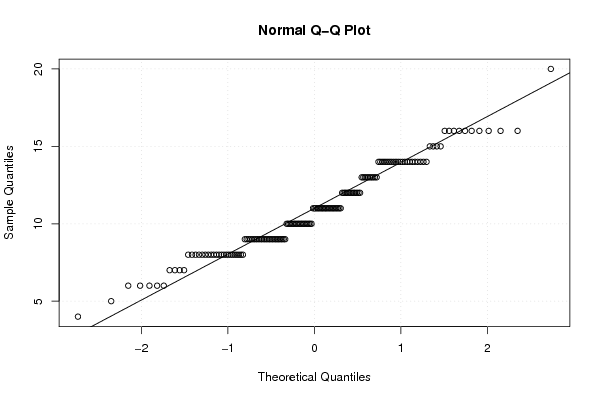
| Title produced by software | Linear Regression Graphical Model Validation | ||||||||||||||||||||||||||||||||||||||||||||||||||||||||||||
| Date of computation | Sun, 14 Nov 2010 12:59:56 +0000 | ||||||||||||||||||||||||||||||||||||||||||||||||||||||||||||
| Cite this page as follows | Statistical Computations at FreeStatistics.org, Office for Research Development and Education, URL https://freestatistics.org/blog/index.php?v=date/2010/Nov/14/t1289739499fq5llck3eubkpo4.htm/, Retrieved Fri, 19 Apr 2024 00:55:39 +0000 | ||||||||||||||||||||||||||||||||||||||||||||||||||||||||||||
| Statistical Computations at FreeStatistics.org, Office for Research Development and Education, URL https://freestatistics.org/blog/index.php?pk=94504, Retrieved Fri, 19 Apr 2024 00:55:39 +0000 | |||||||||||||||||||||||||||||||||||||||||||||||||||||||||||||
| QR Codes: | |||||||||||||||||||||||||||||||||||||||||||||||||||||||||||||
|
| |||||||||||||||||||||||||||||||||||||||||||||||||||||||||||||
| Original text written by user: | |||||||||||||||||||||||||||||||||||||||||||||||||||||||||||||
| IsPrivate? | No (this computation is public) | ||||||||||||||||||||||||||||||||||||||||||||||||||||||||||||
| User-defined keywords | |||||||||||||||||||||||||||||||||||||||||||||||||||||||||||||
| Estimated Impact | 231 | ||||||||||||||||||||||||||||||||||||||||||||||||||||||||||||
Tree of Dependent Computations | |||||||||||||||||||||||||||||||||||||||||||||||||||||||||||||
| Family? (F = Feedback message, R = changed R code, M = changed R Module, P = changed Parameters, D = changed Data) | |||||||||||||||||||||||||||||||||||||||||||||||||||||||||||||
| - [Linear Regression Graphical Model Validation] [Colombia Coffee -...] [2008-02-26 10:22:06] [74be16979710d4c4e7c6647856088456] - M D [Linear Regression Graphical Model Validation] [workshop 6 tutorial] [2010-11-12 10:13:29] [87d60b8864dc39f7ed759c345edfb471] - D [Linear Regression Graphical Model Validation] [workshop 6 mini-t...] [2010-11-12 14:05:27] [87d60b8864dc39f7ed759c345edfb471] - D [Linear Regression Graphical Model Validation] [W6-mini tutorial] [2010-11-12 20:07:18] [48146708a479232c43a8f6e52fbf83b4] - [Linear Regression Graphical Model Validation] [WS 6 - mini-tutor...] [2010-11-13 12:19:57] [033eb2749a430605d9b2be7c4aac4a0c] - P [Linear Regression Graphical Model Validation] [ws 6 mini tutorial] [2010-11-14 12:59:56] [ac4f1d4b47349b2602192853b2bc5b72] [Current] - PD [Linear Regression Graphical Model Validation] [Mini tutorial Par...] [2010-11-15 15:04:36] [d59201e34006b7e3f71c33fa566f42b3] - D [Linear Regression Graphical Model Validation] [Mini tutorial Par...] [2010-11-15 15:52:02] [d59201e34006b7e3f71c33fa566f42b3] | |||||||||||||||||||||||||||||||||||||||||||||||||||||||||||||
| Feedback Forum | |||||||||||||||||||||||||||||||||||||||||||||||||||||||||||||
Post a new message | |||||||||||||||||||||||||||||||||||||||||||||||||||||||||||||
Dataset | |||||||||||||||||||||||||||||||||||||||||||||||||||||||||||||
| Dataseries X: | |||||||||||||||||||||||||||||||||||||||||||||||||||||||||||||
14 11 6 12 8 10 10 11 16 11 13 12 8 12 11 4 9 8 8 14 15 16 9 14 11 8 9 9 9 9 10 16 11 8 9 16 11 16 12 12 14 9 10 9 10 12 14 14 10 14 16 9 10 6 8 13 10 8 7 15 9 10 12 13 10 11 8 9 13 11 8 9 9 15 9 10 14 12 12 11 14 6 12 8 14 11 10 14 12 10 14 5 11 10 9 10 16 13 9 10 10 7 9 8 14 14 8 9 14 14 8 8 8 7 6 8 6 11 14 11 11 11 14 8 20 11 8 11 10 14 11 9 9 8 10 13 13 12 8 13 14 12 14 15 13 16 9 9 9 8 7 16 11 9 11 9 14 13 16 | |||||||||||||||||||||||||||||||||||||||||||||||||||||||||||||
| Dataseries Y: | |||||||||||||||||||||||||||||||||||||||||||||||||||||||||||||
26 23 25 23 19 29 25 21 22 25 24 18 22 15 22 28 20 12 24 20 21 20 21 23 28 24 24 24 23 23 29 24 18 25 21 26 22 22 22 23 30 23 17 23 23 25 24 24 23 21 24 24 28 16 20 29 27 22 28 16 25 24 28 24 23 30 24 21 25 25 22 23 26 23 25 21 25 24 29 22 27 26 22 24 27 24 24 29 22 21 24 24 23 20 27 26 25 21 21 19 21 21 16 22 29 15 17 15 21 21 19 24 20 17 23 24 14 19 24 13 22 16 19 25 25 23 24 26 26 25 18 21 26 23 23 22 20 13 24 15 14 22 10 24 22 24 19 20 13 20 22 24 29 12 20 21 24 22 20 | |||||||||||||||||||||||||||||||||||||||||||||||||||||||||||||
Tables (Output of Computation) | |||||||||||||||||||||||||||||||||||||||||||||||||||||||||||||
| |||||||||||||||||||||||||||||||||||||||||||||||||||||||||||||
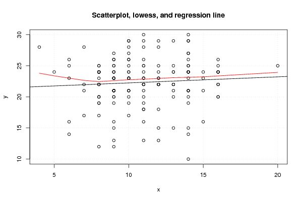
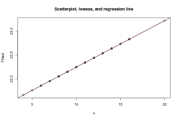
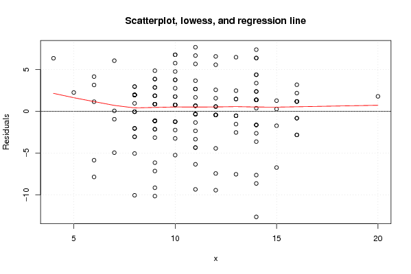
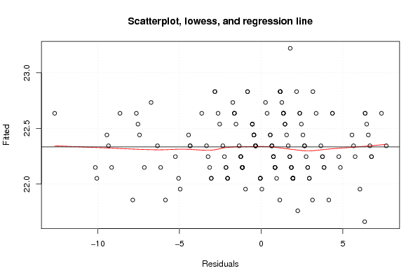
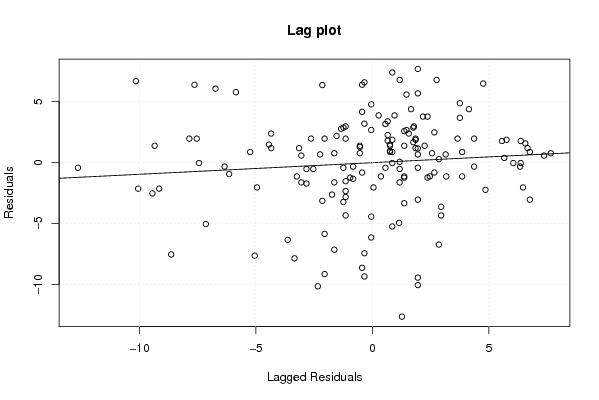
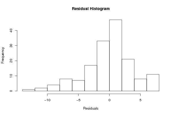
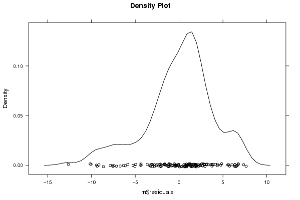
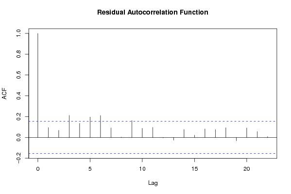
Figures (Output of Computation) | |||||||||||||||||||||||||||||||||||||||||||||||||||||||||||||
Input Parameters & R Code | |||||||||||||||||||||||||||||||||||||||||||||||||||||||||||||
| Parameters (Session): | |||||||||||||||||||||||||||||||||||||||||||||||||||||||||||||
| par1 = 0 ; par2 = 36 ; | |||||||||||||||||||||||||||||||||||||||||||||||||||||||||||||
| Parameters (R input): | |||||||||||||||||||||||||||||||||||||||||||||||||||||||||||||
| par1 = 0 ; | |||||||||||||||||||||||||||||||||||||||||||||||||||||||||||||
| R code (references can be found in the software module): | |||||||||||||||||||||||||||||||||||||||||||||||||||||||||||||
par1 <- as.numeric(par1) | |||||||||||||||||||||||||||||||||||||||||||||||||||||||||||||