Free Statistics

of Irreproducible Research!

Author's title

Author*The author of this computation has been verified*
R Software Modulerwasp_linear_regression.wasp
Title produced by softwareLinear Regression Graphical Model Validation
Date of computationThu, 11 Nov 2010 17:26:19 +0000
Cite this page as followsStatistical Computations at FreeStatistics.org, Office for Research Development and Education, URL https://freestatistics.org/blog/index.php?v=date/2010/Nov/11/t1289496365ox1ynsans8qpjbt.htm/, Retrieved Fri, 19 Apr 2024 06:17:16 +0000
Statistical Computations at FreeStatistics.org, Office for Research Development and Education, URL https://freestatistics.org/blog/index.php?pk=93618, Retrieved Fri, 19 Apr 2024 06:17:16 +0000
QR Codes:

Original text written by user:
IsPrivate?No (this computation is public)
User-defined keywords
Estimated Impact144
Family? (F = Feedback message, R = changed R code, M = changed R Module, P = changed Parameters, D = changed Data)
-     [Linear Regression Graphical Model Validation] [shwws4vr1] [2009-10-28 17:20:10] [2b2cfeea2f5ac2a1bcb842baaf1415ef]
-  MPD    [Linear Regression Graphical Model Validation] [Enkelvoudige line...] [2010-11-11 17:26:19] [b6992a7b26e556359948e164e4227eba] [Current]
Feedback Forum

Post a new message
Dataseries X:
1280
1024
1120
1024
1280
1280
1280
1024
1280
1280
1280
1280
1280
1688
1440
1600
1280
1280
1280
1176
1280
1503
1440
1366
1280
1024
1280
2560
1280
1024
1280
1280
1440
1280
1440
1024
1440
1143
1280
1440
1280
1366
1024
1408
1366
1176
1920
1257
1280
1280
1440
1680
1440
1024
1140
1280
1280
1280
1280
1280
1440
1280
1152
1280
1280
1440
1280
1280
1440
1280
1280
1440
1280
1280
1600
1024
1366
1280
1280
1440
1366
1280
1024
1280
1440
1280
1280
1408
1280
1600
1600
1680
1440
1440
917
1280
1760
1280
1280
1280
1024
1366
1440
1280
1280
1920
1024
1024
1600
1117
1440
983
1024
1024
1280
1440
1280
1280
1280
1440
1280
1024
1024
1152
1280
1024
1366
1680
1680
1280
1366
1024
1440
1024
1280
1280
1280
1024
1280
Dataseries Y:
1024
768
700
768
800
1024
800
768
800
1024
800
800
1024
949
900
1200
800
800
768
735
800
845
900
768
768
768
800
1440
768
768
1024
800
900
800
900
768
900
857
800
900
800
768
768
880
768
735
1200
785
800
800
900
1050
900
768
641
1024
800
800
800
800
900
800
864
1024
800
900
800
1024
900
800
800
900
800
1024
900
768
768
800
800
900
768
800
768
800
900
800
800
880
800
900
900
1050
900
900
550
800
990
800
800
800
768
768
900
800
1024
1080
768
768
900
698
900
737
768
640
800
900
800
800
800
900
800
768
768
864
768
768
768
1050
1050
800
768
768
900
768
800
800
800
768
800


Summary of computational transaction
Raw Inputview raw input (R code)
Raw Outputview raw output of R engine
Computing time5 seconds
R Server'Sir Ronald Aylmer Fisher' @ 193.190.124.24

\begin{tabular}{lllllllll}
\hline
Summary of computational transaction \tabularnewline
Raw Input & view raw input (R code)  \tabularnewline
Raw Output & view raw output of R engine  \tabularnewline
Computing time & 5 seconds \tabularnewline
R Server & 'Sir Ronald Aylmer Fisher' @ 193.190.124.24 \tabularnewline
\hline
\end{tabular}
%Source: https://freestatistics.org/blog/index.php?pk=93618&T=0

[TABLE]
[ROW][C]Summary of computational transaction[/C][/ROW]
[ROW][C]Raw Input[/C][C]view raw input (R code) [/C][/ROW]
[ROW][C]Raw Output[/C][C]view raw output of R engine [/C][/ROW]
[ROW][C]Computing time[/C][C]5 seconds[/C][/ROW]
[ROW][C]R Server[/C][C]'Sir Ronald Aylmer Fisher' @ 193.190.124.24[/C][/ROW]
[/TABLE]
Source: https://freestatistics.org/blog/index.php?pk=93618&T=0

Globally Unique Identifier (entire table): ba.freestatistics.org/blog/index.php?pk=93618&T=0

As an alternative you can also use a QR Code:  

The GUIDs for individual cells are displayed in the table below:

Summary of computational transaction
Raw Inputview raw input (R code)
Raw Outputview raw output of R engine
Computing time5 seconds
R Server'Sir Ronald Aylmer Fisher' @ 193.190.124.24


Simple Linear Regression
StatisticsEstimateS.D.T-STAT (H0: coeff=0)P-value (two-sided)
constant term308.04953567382538.77752565475887.944022483962226.39266417579165e-13
slope0.4097724624741070.029235746183536414.01614516358280

\begin{tabular}{lllllllll}
\hline
Simple Linear Regression \tabularnewline
Statistics & Estimate & S.D. & T-STAT (H0: coeff=0) & P-value (two-sided) \tabularnewline
constant term & 308.049535673825 & 38.7775256547588 & 7.94402248396222 & 6.39266417579165e-13 \tabularnewline
slope & 0.409772462474107 & 0.0292357461835364 & 14.0161451635828 & 0 \tabularnewline
\hline
\end{tabular}
%Source: https://freestatistics.org/blog/index.php?pk=93618&T=1

[TABLE]
[ROW][C]Simple Linear Regression[/C][/ROW]
[ROW][C]Statistics[/C][C]Estimate[/C][C]S.D.[/C][C]T-STAT (H0: coeff=0)[/C][C]P-value (two-sided)[/C][/ROW]
[ROW][C]constant term[/C][C]308.049535673825[/C][C]38.7775256547588[/C][C]7.94402248396222[/C][C]6.39266417579165e-13[/C][/ROW]
[ROW][C]slope[/C][C]0.409772462474107[/C][C]0.0292357461835364[/C][C]14.0161451635828[/C][C]0[/C][/ROW]
[/TABLE]
Source: https://freestatistics.org/blog/index.php?pk=93618&T=1

Globally Unique Identifier (entire table): ba.freestatistics.org/blog/index.php?pk=93618&T=1

As an alternative you can also use a QR Code:  

The GUIDs for individual cells are displayed in the table below:

Simple Linear Regression
StatisticsEstimateS.D.T-STAT (H0: coeff=0)P-value (two-sided)
constant term308.04953567382538.77752565475887.944022483962226.39266417579165e-13
slope0.4097724624741070.029235746183536414.01614516358280


Parameters (Session):
par2 = grey ; par3 = FALSE ; par4 = Unknown ;
Parameters (R input):
par1 = 0 ;
R code (references can be found in the software module):
par1 <- as.numeric(par1)
library(lattice)
z <- as.data.frame(cbind(x,y))
m <- lm(y~x)
summary(m)
bitmap(file='test1.png')
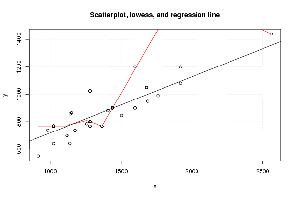
plot(z,main='Scatterplot, lowess, and regression line')
lines(lowess(z),col='red')
abline(m)
grid()
dev.off()
bitmap(file='test2.png')
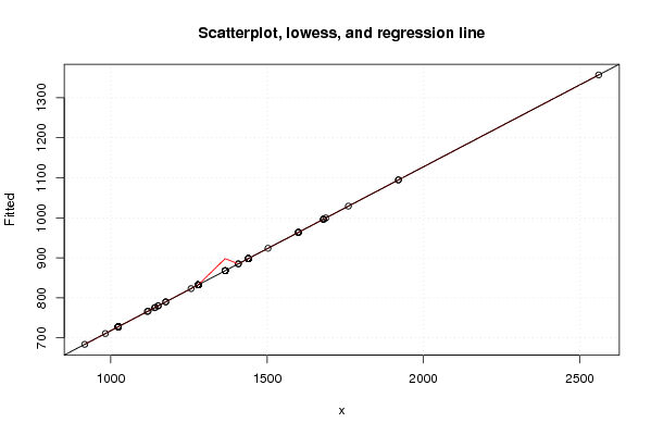
m2 <- lm(m$fitted.values ~ x)
summary(m2)
z2 <- as.data.frame(cbind(x,m$fitted.values))
names(z2) <- list('x','Fitted')
plot(z2,main='Scatterplot, lowess, and regression line')
lines(lowess(z2),col='red')
abline(m2)
grid()
dev.off()
bitmap(file='test3.png')
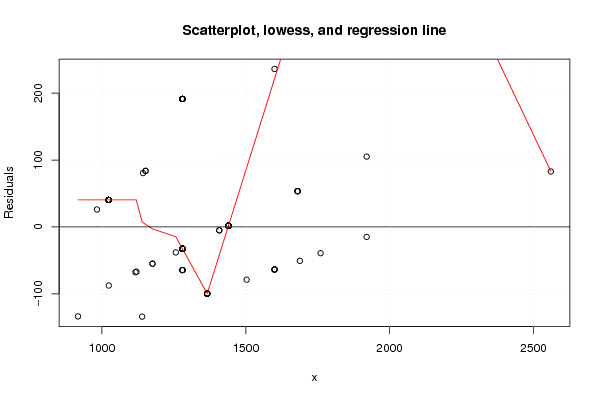
m3 <- lm(m$residuals ~ x)
summary(m3)
z3 <- as.data.frame(cbind(x,m$residuals))
names(z3) <- list('x','Residuals')
plot(z3,main='Scatterplot, lowess, and regression line')
lines(lowess(z3),col='red')
abline(m3)
grid()
dev.off()
bitmap(file='test4.png')
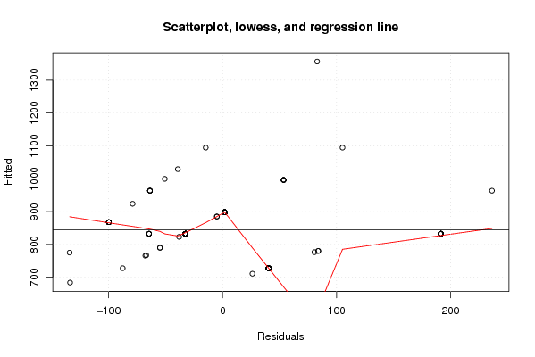
m4 <- lm(m$fitted.values ~ m$residuals)
summary(m4)
z4 <- as.data.frame(cbind(m$residuals,m$fitted.values))
names(z4) <- list('Residuals','Fitted')
plot(z4,main='Scatterplot, lowess, and regression line')
lines(lowess(z4),col='red')
abline(m4)
grid()
dev.off()
bitmap(file='test5.png')
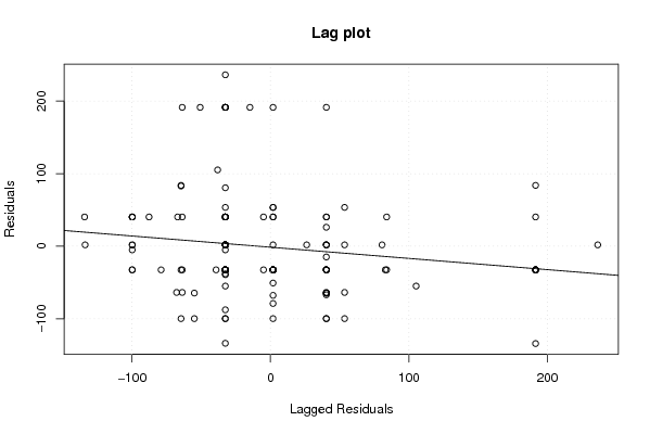
myr <- as.ts(m$residuals)
z5 <- as.data.frame(cbind(lag(myr,1),myr))
names(z5) <- list('Lagged Residuals','Residuals')
plot(z5,main='Lag plot')
m5 <- lm(z5)
summary(m5)
abline(m5)
grid()
dev.off()
bitmap(file='test6.png')
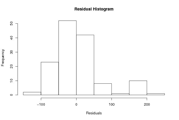
hist(m$residuals,main='Residual Histogram',xlab='Residuals')
dev.off()
bitmap(file='test7.png')
if (par1 > 0)
{
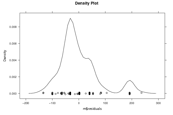
densityplot(~m$residuals,col='black',main=paste('Density Plot bw = ',par1),bw=par1)
} else {
densityplot(~m$residuals,col='black',main='Density Plot')
}
dev.off()
bitmap(file='test8.png')
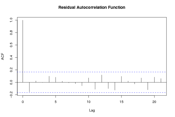
acf(m$residuals,main='Residual Autocorrelation Function')
dev.off()
bitmap(file='test9.png')
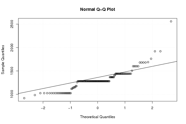
qqnorm(x)
qqline(x)
grid()
dev.off()
load(file='createtable')
a<-table.start()
a<-table.row.start(a)
a<-table.element(a,'Simple Linear Regression',5,TRUE)
a<-table.row.end(a)
a<-table.row.start(a)
a<-table.element(a,'Statistics',1,TRUE)
a<-table.element(a,'Estimate',1,TRUE)
a<-table.element(a,'S.D.',1,TRUE)
a<-table.element(a,'T-STAT (H0: coeff=0)',1,TRUE)
a<-table.element(a,'P-value (two-sided)',1,TRUE)
a<-table.row.end(a)
a<-table.row.start(a)
a<-table.element(a,'constant term',header=TRUE)
a<-table.element(a,m$coefficients[[1]])
sd <- sqrt(vcov(m)[1,1])
a<-table.element(a,sd)
tstat <- m$coefficients[[1]]/sd
a<-table.element(a,tstat)
pval <- 2*(1-pt(abs(tstat),length(x)-2))
a<-table.element(a,pval)
a<-table.row.end(a)
a<-table.row.start(a)
a<-table.element(a,'slope',header=TRUE)
a<-table.element(a,m$coefficients[[2]])
sd <- sqrt(vcov(m)[2,2])
a<-table.element(a,sd)
tstat <- m$coefficients[[2]]/sd
a<-table.element(a,tstat)
pval <- 2*(1-pt(abs(tstat),length(x)-2))
a<-table.element(a,pval)
a<-table.row.end(a)
a<-table.end(a)
table.save(a,file='mytable.tab')