Repository of Reproducible Computations

Free Statistics

of Irreproducible Research!

Author's title

Author

*The author of this computation has been verified*

R Software Module

rwasp_bootstrapplot.wasp

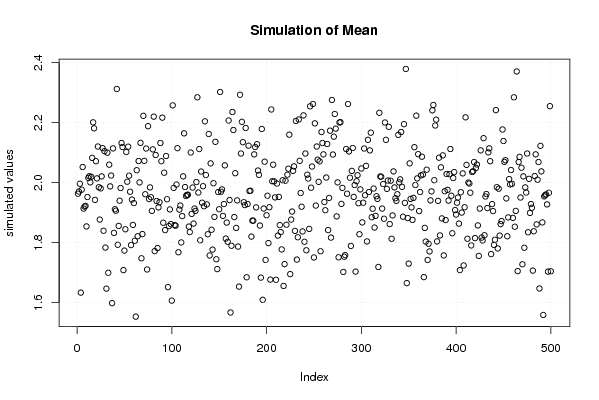
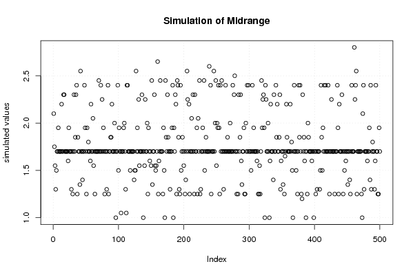
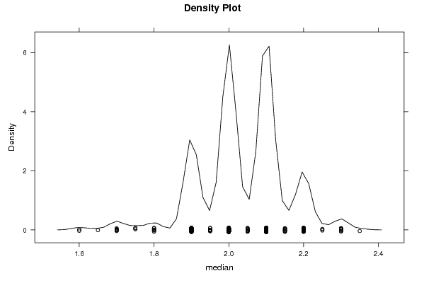
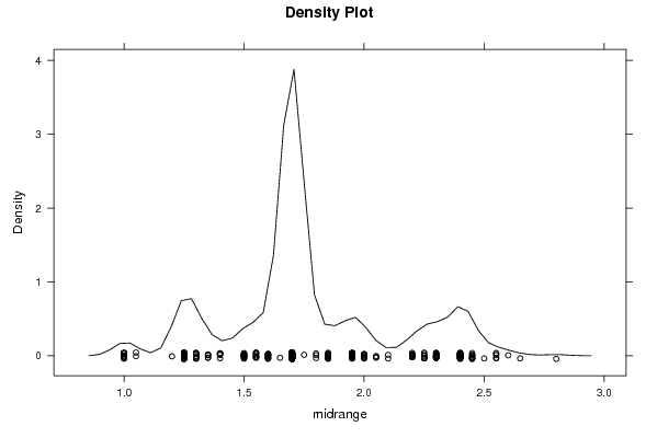
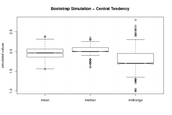
Title produced by software

Blocked Bootstrap Plot - Central Tendency

Date of computation

Thu, 11 Nov 2010 17:13:44 +0000

Cite this page as follows

Statistical Computations at FreeStatistics.org, Office for Research Development and Education, URL https://freestatistics.org/blog/index.php?v=date/2010/Nov/11/t1289495546kslf8sanp6i2o98.htm/, Retrieved Thu, 25 Apr 2024 16:01:25 +0000

Statistical Computations at FreeStatistics.org, Office for Research Development and Education, URL https://freestatistics.org/blog/index.php?pk=93606, Retrieved Thu, 25 Apr 2024 16:01:25 +0000

QR Codes:

Paste this QR Code to cite your computation.

Original text written by user:

IsPrivate?

No (this computation is public)

User-defined keywords

Estimated Impact

152

Family? (F = Feedback message, R = changed R code, M = changed R Module, P = changed Parameters, D = changed Data)

-     [Bivariate Data Series] [Bivariate dataset] [2008-01-05 23:51:08] [74be16979710d4c4e7c6647856088456]
- RMPD  [Blocked Bootstrap Plot - Central Tendency] [Colombia Coffee] [2008-01-07 10:26:26] [74be16979710d4c4e7c6647856088456]
- RM D      [Blocked Bootstrap Plot - Central Tendency] [WS6 - Mini Tutori...] [2010-11-11 17:13:44] [ee4a783fb13f41eb2e9bc8a0c4f26279] [Current]
-    D        [Blocked Bootstrap Plot - Central Tendency] [WS6 - Mini Tutori...] [2010-11-16 18:10:05] [1f5baf2b24e732d76900bb8178fc04e7] 

Feedback Forum

Post a new message

Dataseries X:

Download CSV

Histogram

Boxplots

2,4
2,4
2,5
2,6
2,4
2,6
2,4
2,3
2,4
2,4
2,4
2,4
2,4
2,4
2,4
2,4
2,5
2,1
2,1
2
2
2
1,9
1,9
2
1,8
1,6
1,3
1,4
1,4
1,5
1,7
1,6
1,5
1,6
1,5
1,1
1,1
1,1
1,4
1,3
1,4
1,3
1,1
1
0,9
0,8
0,8
0,8
0,8
1
1,1
1
0,9
1,1
1,2
1,2
1,4
1,5
1,7
1,9
1,9
1,9
1,7
1,7
2,1
2
2
2,5
2,4
2,5
2,5
2
1,9
2,2
2,7
3,1
2,8
2,6
2,3
2,2
2,2
2
2
2,6
2,5
2,5
2,3
2
1,9
2
2,1
2,1
2,3
2,3
2,3
2,1
2,4
2,5
2,1
1,8
1,9
1,9
2,1
2,2
2
2,2
2
1,9
1,6
1,7
2
2,5
2,4
2,3
2,3
2,1
2,4
2,2
2,4
1,9
2,1
2,1
2,1
2
2,1
2,2
2,2
2,6
2,5
2,3
2,2
2,4
2,3
2,2
2,5
2,5
2,5
2,4
2,3
1,7
1,6
1,9
1,9
1,8
1,8
1,9
1,9
1,9
1,9
1,8
1,7
2,1
2,6
3,1
3,1
3,2
3,3
3,6
3,3
3,7
4
4
3,8
3,6
3,2
2,1
1,6
1,1
1,2
0,6
0,6
0
-0,1
-0,6
-0,2
-0,3
-0,1
0,5
0,9

Summary of computational transaction
Raw Input	view raw input (R code)
Raw Output	view raw output of R engine
Computing time	3 seconds
R Server	'George Udny Yule' @ 72.249.76.132

\begin{tabular}{lllllllll}
\hline
Summary of computational transaction \tabularnewline
Raw Input & view raw input (R code)  \tabularnewline
Raw Output & view raw output of R engine  \tabularnewline
Computing time & 3 seconds \tabularnewline
R Server & 'George Udny Yule' @ 72.249.76.132 \tabularnewline
\hline
\end{tabular}
%Source: https://freestatistics.org/blog/index.php?pk=93606&T=0

[TABLE]
[ROW][C]Summary of computational transaction[/C][/ROW]
[ROW][C]Raw Input[/C][C]view raw input (R code) [/C][/ROW]
[ROW][C]Raw Output[/C][C]view raw output of R engine [/C][/ROW]
[ROW][C]Computing time[/C][C]3 seconds[/C][/ROW]
[ROW][C]R Server[/C][C]'George Udny Yule' @ 72.249.76.132[/C][/ROW]
[/TABLE]
Source: https://freestatistics.org/blog/index.php?pk=93606&T=0

Globally Unique Identifier (entire table): ba.freestatistics.org/blog/index.php?pk=93606&T=0

As an alternative you can also use a QR Code:

The GUIDs for individual cells are displayed in the table below:

Summary of computational transaction
Raw Input	view raw input (R code)
Raw Output	view raw output of R engine
Computing time	3 seconds
R Server	'George Udny Yule' @ 72.249.76.132

Estimation Results of Blocked Bootstrap
statistic	Q1	Estimate	Q3	S.D.	IQR
mean	1.86027777777778	1.96277777777778	2.06388888888889	0.150002521643533	0.203611111111111
median	2	2	2.1	0.114223877487926	0.1
midrange	1.7	1.7	1.95	0.347101640875114	0.25

\begin{tabular}{lllllllll}
\hline
Estimation Results of Blocked Bootstrap \tabularnewline
statistic & Q1 & Estimate & Q3 & S.D. & IQR \tabularnewline
mean & 1.86027777777778 & 1.96277777777778 & 2.06388888888889 & 0.150002521643533 & 0.203611111111111 \tabularnewline
median & 2 & 2 & 2.1 & 0.114223877487926 & 0.1 \tabularnewline
midrange & 1.7 & 1.7 & 1.95 & 0.347101640875114 & 0.25 \tabularnewline
\hline
\end{tabular}
%Source: https://freestatistics.org/blog/index.php?pk=93606&T=1

[TABLE]
[ROW][C]Estimation Results of Blocked Bootstrap[/C][/ROW]
[ROW][C]statistic[/C][C]Q1[/C][C]Estimate[/C][C]Q3[/C][C]S.D.[/C][C]IQR[/C][/ROW]
[ROW][C]mean[/C][C]1.86027777777778[/C][C]1.96277777777778[/C][C]2.06388888888889[/C][C]0.150002521643533[/C][C]0.203611111111111[/C][/ROW]
[ROW][C]median[/C][C]2[/C][C]2[/C][C]2.1[/C][C]0.114223877487926[/C][C]0.1[/C][/ROW]
[ROW][C]midrange[/C][C]1.7[/C][C]1.7[/C][C]1.95[/C][C]0.347101640875114[/C][C]0.25[/C][/ROW]
[/TABLE]
Source: https://freestatistics.org/blog/index.php?pk=93606&T=1

Globally Unique Identifier (entire table): ba.freestatistics.org/blog/index.php?pk=93606&T=1

As an alternative you can also use a QR Code:

The GUIDs for individual cells are displayed in the table below:

Estimation Results of Blocked Bootstrap
statistic	Q1	Estimate	Q3	S.D.	IQR
mean	1.86027777777778	1.96277777777778	2.06388888888889	0.150002521643533	0.203611111111111
median	2	2	2.1	0.114223877487926	0.1
midrange	1.7	1.7	1.95	0.347101640875114	0.25

Figure 1

PNG link

Postscript link

PDF link

Figure 2

PNG link

Postscript link

PDF link

Figure 3

PNG link

Postscript link

PDF link

Figure 4

PNG link

Postscript link

PDF link

Figure 5

PNG link

Postscript link

PDF link

Figure 6

PNG link

Postscript link

PDF link

Figure 7

PNG link

Postscript link

PDF link

Parameters (Session):

par1 = 500 ; par2 = 12 ;

Parameters (R input):

par1 = 500 ; par2 = 12 ;

R code (references can be found in the software module):

par1 <- as.numeric(par1)
par2 <- as.numeric(par2)
if (par1 < 10) par1 = 10
if (par1 > 5000) par1 = 5000
if (par2 < 3) par2 = 3
if (par2 > length(x)) par2 = length(x)
library(lattice)
library(boot)
boot.stat <- function(s)
{
s.mean <- mean(s)
s.median <- median(s)
s.midrange <- (max(s) + min(s)) / 2
c(s.mean, s.median, s.midrange)
}
(r <- tsboot(x, boot.stat, R=par1, l=12, sim='fixed'))
bitmap(file='plot1.png')
plot(r$t[,1],type='p',ylab='simulated values',main='Simulation of Mean')
grid()
dev.off()
bitmap(file='plot2.png')
plot(r$t[,2],type='p',ylab='simulated values',main='Simulation of Median')
grid()
dev.off()
bitmap(file='plot3.png')
plot(r$t[,3],type='p',ylab='simulated values',main='Simulation of Midrange')
grid()
dev.off()
bitmap(file='plot4.png')
densityplot(~r$t[,1],col='black',main='Density Plot',xlab='mean')
dev.off()
bitmap(file='plot5.png')
densityplot(~r$t[,2],col='black',main='Density Plot',xlab='median')
dev.off()
bitmap(file='plot6.png')
densityplot(~r$t[,3],col='black',main='Density Plot',xlab='midrange')
dev.off()
z <- data.frame(cbind(r$t[,1],r$t[,2],r$t[,3]))
colnames(z) <- list('mean','median','midrange')
bitmap(file='plot7.png')
boxplot(z,notch=TRUE,ylab='simulated values',main='Bootstrap Simulation - Central Tendency')
grid()
dev.off()
load(file='createtable')
a<-table.start()
a<-table.row.start(a)
a<-table.element(a,'Estimation Results of Blocked Bootstrap',6,TRUE)
a<-table.row.end(a)
a<-table.row.start(a)
a<-table.element(a,'statistic',header=TRUE)
a<-table.element(a,'Q1',header=TRUE)
a<-table.element(a,'Estimate',header=TRUE)
a<-table.element(a,'Q3',header=TRUE)
a<-table.element(a,'S.D.',header=TRUE)
a<-table.element(a,'IQR',header=TRUE)
a<-table.row.end(a)
a<-table.row.start(a)
a<-table.element(a,'mean',header=TRUE)
q1 <- quantile(r$t[,1],0.25)[[1]]
q3 <- quantile(r$t[,1],0.75)[[1]]
a<-table.element(a,q1)
a<-table.element(a,r$t0[1])
a<-table.element(a,q3)
a<-table.element(a,sqrt(var(r$t[,1])))
a<-table.element(a,q3-q1)
a<-table.row.end(a)
a<-table.row.start(a)
a<-table.element(a,'median',header=TRUE)
q1 <- quantile(r$t[,2],0.25)[[1]]
q3 <- quantile(r$t[,2],0.75)[[1]]
a<-table.element(a,q1)
a<-table.element(a,r$t0[2])
a<-table.element(a,q3)
a<-table.element(a,sqrt(var(r$t[,2])))
a<-table.element(a,q3-q1)
a<-table.row.end(a)
a<-table.row.start(a)
a<-table.element(a,'midrange',header=TRUE)
q1 <- quantile(r$t[,3],0.25)[[1]]
q3 <- quantile(r$t[,3],0.75)[[1]]
a<-table.element(a,q1)
a<-table.element(a,r$t0[3])
a<-table.element(a,q3)
a<-table.element(a,sqrt(var(r$t[,3])))
a<-table.element(a,q3-q1)
a<-table.row.end(a)
a<-table.end(a)
table.save(a,file='mytable.tab')

Free Statistics

Description of Statistical Computation

Tree of Dependent Computations

Dataset

Tables (Output of Computation)

Figures (Output of Computation)

Input Parameters & R Code