Free Statistics
of Irreproducible Research!
Description of Statistical Computation | |||||||||||||||||||||
|---|---|---|---|---|---|---|---|---|---|---|---|---|---|---|---|---|---|---|---|---|---|
| Author's title | |||||||||||||||||||||
| Author | *The author of this computation has been verified* | ||||||||||||||||||||
| R Software Module | rwasp_meanplot.wasp | ||||||||||||||||||||
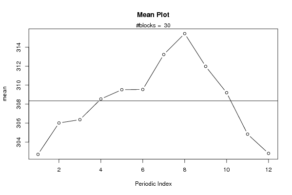
| Title produced by software | Mean Plot | ||||||||||||||||||||
| Date of computation | Thu, 11 Nov 2010 14:01:36 +0000 | ||||||||||||||||||||
| Cite this page as follows | Statistical Computations at FreeStatistics.org, Office for Research Development and Education, URL https://freestatistics.org/blog/index.php?v=date/2010/Nov/11/t1289484113gzzcoqtng3xjom8.htm/, Retrieved Fri, 26 Apr 2024 18:56:41 +0000 | ||||||||||||||||||||
| Statistical Computations at FreeStatistics.org, Office for Research Development and Education, URL https://freestatistics.org/blog/index.php?pk=93383, Retrieved Fri, 26 Apr 2024 18:56:41 +0000 | |||||||||||||||||||||
| QR Codes: | |||||||||||||||||||||
|
| |||||||||||||||||||||
| Original text written by user: | |||||||||||||||||||||
| IsPrivate? | No (this computation is public) | ||||||||||||||||||||
| User-defined keywords | |||||||||||||||||||||
| Estimated Impact | 114 | ||||||||||||||||||||
Tree of Dependent Computations | |||||||||||||||||||||
| Family? (F = Feedback message, R = changed R code, M = changed R Module, P = changed Parameters, D = changed Data) | |||||||||||||||||||||
| - [Bivariate Data Series] [Bivariate dataset] [2008-01-05 23:51:08] [74be16979710d4c4e7c6647856088456] F RMPD [Mean Plot] [Colombia Coffee] [2008-01-07 13:38:24] [74be16979710d4c4e7c6647856088456] - MPD [Mean Plot] [ws 6 - Q3 - Seaso...] [2010-11-11 14:01:36] [0829c729852d8a4b1b0c41cf0848af95] [Current] | |||||||||||||||||||||
| Feedback Forum | |||||||||||||||||||||
Post a new message | |||||||||||||||||||||
Dataset | |||||||||||||||||||||
| Dataseries X: | |||||||||||||||||||||
255,00 280,20 299,90 339,20 374,20 393,50 389,20 381,70 375,20 369,00 357,40 352,10 346,50 342,90 340,30 328,30 322,90 314,30 308,90 294,00 285,60 281,20 280,30 278,80 274,50 270,40 263,40 259,90 258,00 262,70 284,70 311,30 322,10 327,00 331,30 333,30 321,40 327,00 320,00 314,70 316,70 314,40 321,30 318,20 307,20 301,30 287,50 277,70 274,40 258,80 253,30 251,00 248,40 249,50 246,10 244,50 243,60 244,00 240,80 249,80 248,00 259,40 260,50 260,80 261,30 259,50 256,60 257,90 256,50 254,20 253,30 253,80 255,50 257,10 257,30 253,20 252,80 252,00 250,70 252,20 250,00 251,00 253,40 251,20 255,60 261,10 258,90 259,90 261,20 264,70 267,10 266,40 267,70 268,60 267,50 268,50 268,50 270,50 270,90 270,10 269,30 269,80 270,10 264,90 263,70 264,80 263,70 255,90 276,20 360,10 380,50 373,70 369,80 366,60 359,30 345,80 326,20 324,50 328,10 327,50 324,40 316,50 310,90 301,50 291,70 290,40 287,40 277,70 281,60 288,00 276,00 272,90 283,00 283,30 276,80 284,50 282,70 281,20 287,40 283,10 284,00 285,50 289,20 292,50 296,40 305,20 303,90 311,50 316,30 316,70 322,50 317,10 309,80 303,80 290,30 293,70 291,70 296,50 289,10 288,50 293,80 297,70 305,40 302,70 302,50 303,00 294,50 294,10 294,50 297,10 289,40 292,40 287,90 286,60 280,50 272,40 269,20 270,60 267,30 262,50 266,80 268,80 263,10 261,20 266,00 262,50 265,20 261,30 253,70 249,20 239,10 236,40 235,20 245,20 246,20 247,70 251,40 253,30 254,80 250,00 249,30 241,50 243,30 248,00 253,00 252,90 251,50 251,60 253,50 259,80 334,10 448,00 445,80 445,00 448,20 438,20 439,80 423,40 410,80 408,40 406,70 405,90 402,70 405,10 399,60 386,50 381,40 375,20 357,70 359,00 355,00 352,70 344,40 343,80 338,00 339,00 333,30 334,40 328,30 330,70 330,00 331,60 351,20 389,40 410,90 442,80 462,80 466,90 461,70 439,20 430,30 416,10 402,50 397,30 403,30 395,90 387,80 378,60 377,10 370,40 362,00 350,30 348,20 344,60 343,50 342,80 347,60 346,60 349,50 342,10 342,00 342,80 339,30 348,20 333,70 334,70 354,00 367,70 363,30 358,40 353,10 343,10 344,60 344,40 333,90 331,70 324,30 321,20 322,40 321,70 320,50 312,80 309,70 315,60 309,70 304,60 302,50 301,50 298,80 291,30 293,60 294,60 285,90 297,60 301,10 293,80 297,70 292,90 292,10 287,20 288,20 283,80 299,90 292,40 293,30 300,80 293,70 293,10 294,40 292,10 291,90 282,50 277,90 287,50 289,20 285,60 293,20 290,80 283,10 275,00 287,80 287,80 287,40 284,00 277,80 277,60 304,90 294,00 300,90 324,00 332,90 341,60 333,40 348,20 344,70 344,70 329,30 323,50 323,20 317,40 330,10 329,20 334,90 315,80 315,40 319,60 317,30 313,80 315,80 311,30 | |||||||||||||||||||||
Tables (Output of Computation) | |||||||||||||||||||||
| |||||||||||||||||||||
Figures (Output of Computation) | |||||||||||||||||||||
Input Parameters & R Code | |||||||||||||||||||||
| Parameters (Session): | |||||||||||||||||||||
| par1 = 12 ; | |||||||||||||||||||||
| Parameters (R input): | |||||||||||||||||||||
| par1 = 12 ; | |||||||||||||||||||||
| R code (references can be found in the software module): | |||||||||||||||||||||
par1 <- as.numeric(par1) | |||||||||||||||||||||