Free Statistics
of Irreproducible Research!
Description of Statistical Computation | |||||||||||||||||||||||||||||||||||||||||||||||||||||
|---|---|---|---|---|---|---|---|---|---|---|---|---|---|---|---|---|---|---|---|---|---|---|---|---|---|---|---|---|---|---|---|---|---|---|---|---|---|---|---|---|---|---|---|---|---|---|---|---|---|---|---|---|---|
| Author's title | |||||||||||||||||||||||||||||||||||||||||||||||||||||
| Author | *The author of this computation has been verified* | ||||||||||||||||||||||||||||||||||||||||||||||||||||
| R Software Module | rwasp_edauni.wasp | ||||||||||||||||||||||||||||||||||||||||||||||||||||
| Title produced by software | Univariate Explorative Data Analysis | ||||||||||||||||||||||||||||||||||||||||||||||||||||
| Date of computation | Thu, 11 Nov 2010 13:16:21 +0000 | ||||||||||||||||||||||||||||||||||||||||||||||||||||
| Cite this page as follows | Statistical Computations at FreeStatistics.org, Office for Research Development and Education, URL https://freestatistics.org/blog/index.php?v=date/2010/Nov/11/t12894812821n2dbh5n59u2553.htm/, Retrieved Thu, 18 Apr 2024 22:36:05 +0000 | ||||||||||||||||||||||||||||||||||||||||||||||||||||
| Statistical Computations at FreeStatistics.org, Office for Research Development and Education, URL https://freestatistics.org/blog/index.php?pk=93293, Retrieved Thu, 18 Apr 2024 22:36:05 +0000 | |||||||||||||||||||||||||||||||||||||||||||||||||||||
| QR Codes: | |||||||||||||||||||||||||||||||||||||||||||||||||||||
|
| |||||||||||||||||||||||||||||||||||||||||||||||||||||
| Original text written by user: | |||||||||||||||||||||||||||||||||||||||||||||||||||||
| IsPrivate? | No (this computation is public) | ||||||||||||||||||||||||||||||||||||||||||||||||||||
| User-defined keywords | |||||||||||||||||||||||||||||||||||||||||||||||||||||
| Estimated Impact | 214 | ||||||||||||||||||||||||||||||||||||||||||||||||||||
Tree of Dependent Computations | |||||||||||||||||||||||||||||||||||||||||||||||||||||
| Family? (F = Feedback message, R = changed R code, M = changed R Module, P = changed Parameters, D = changed Data) | |||||||||||||||||||||||||||||||||||||||||||||||||||||
| - [Bivariate Data Series] [Bivariate dataset] [2008-01-05 23:51:08] [74be16979710d4c4e7c6647856088456] F RMPD [Univariate Explorative Data Analysis] [Colombia Coffee] [2008-01-07 14:21:11] [74be16979710d4c4e7c6647856088456] - MPD [Univariate Explorative Data Analysis] [Mini tutorial 2] [2010-11-11 13:16:21] [380f6bceef280be3d93cc6fafd18141e] [Current] - D [Univariate Explorative Data Analysis] [ws6 mini tutorial...] [2010-11-15 17:46:29] [e4076051fbfb461c886b1e223cd7862f] - D [Univariate Explorative Data Analysis] [ws6.mini hypothese 2] [2010-11-15 18:19:49] [e4076051fbfb461c886b1e223cd7862f] - D [Univariate Explorative Data Analysis] [] [2010-11-16 13:16:37] [8d09066a9d3795298da6860e7d4a4400] - [Univariate Explorative Data Analysis] [] [2010-11-17 06:00:13] [6e5489189f7de5cfbcc25dd35ae15009] - D [Univariate Explorative Data Analysis] [] [2010-11-16 13:26:20] [8d09066a9d3795298da6860e7d4a4400] - [Univariate Explorative Data Analysis] [] [2010-11-17 06:01:04] [6e5489189f7de5cfbcc25dd35ae15009] - RM [Univariate Explorative Data Analysis] [mini tuorial] [2011-11-15 15:20:34] [d31984dff2665bea309b726bae3d5241] - R D [Univariate Explorative Data Analysis] [] [2011-11-15 17:03:59] [ad2d4c5ace9fa07b356a7b5098237581] - R D [Univariate Explorative Data Analysis] [Graph Mini-Tutorial] [2011-11-15 22:12:51] [f722e8e78b9e5c5ebaa2263f273aa636] | |||||||||||||||||||||||||||||||||||||||||||||||||||||
| Feedback Forum | |||||||||||||||||||||||||||||||||||||||||||||||||||||
Post a new message | |||||||||||||||||||||||||||||||||||||||||||||||||||||
Dataset | |||||||||||||||||||||||||||||||||||||||||||||||||||||
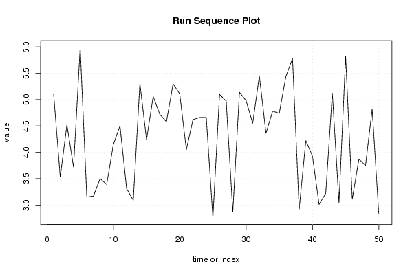
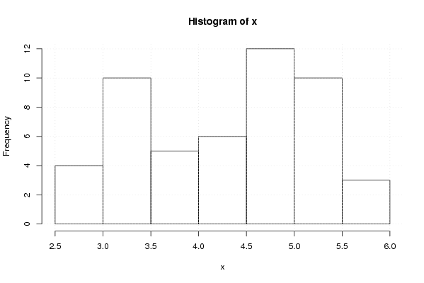
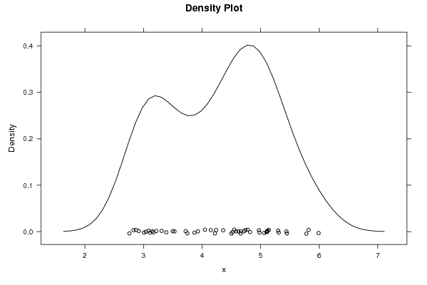
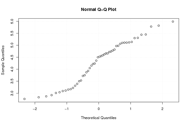
| Dataseries X: | |||||||||||||||||||||||||||||||||||||||||||||||||||||
5,11 3,53 4,52 3,72 5,99 3,15 3,17 3,50 3,39 4,15 4,50 3,31 3,09 5,31 4,24 5,06 4,72 4,58 5,30 5,11 4,05 4,62 4,66 4,66 2,76 5,10 4,97 2,87 5,14 4,98 4,55 5,45 4,36 4,78 4,74 5,44 5,78 2,92 4,22 3,93 3,01 3,22 5,12 3,04 5,82 3,11 3,87 3,75 4,82 2,83 | |||||||||||||||||||||||||||||||||||||||||||||||||||||
Tables (Output of Computation) | |||||||||||||||||||||||||||||||||||||||||||||||||||||
| |||||||||||||||||||||||||||||||||||||||||||||||||||||
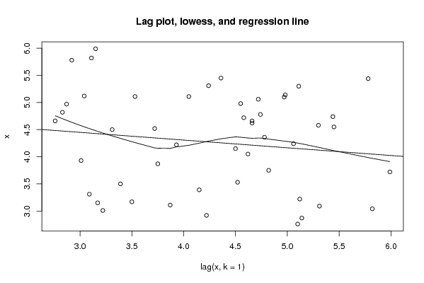
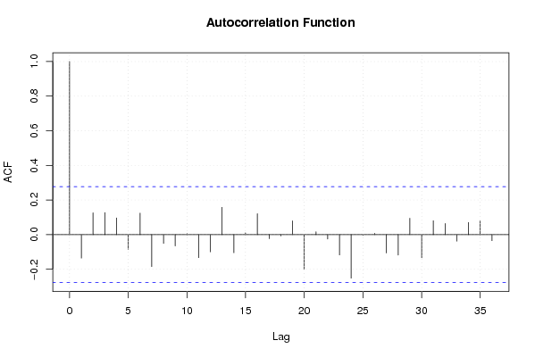
Figures (Output of Computation) | |||||||||||||||||||||||||||||||||||||||||||||||||||||
Input Parameters & R Code | |||||||||||||||||||||||||||||||||||||||||||||||||||||
| Parameters (Session): | |||||||||||||||||||||||||||||||||||||||||||||||||||||
| par1 = 0 ; par2 = 36 ; | |||||||||||||||||||||||||||||||||||||||||||||||||||||
| Parameters (R input): | |||||||||||||||||||||||||||||||||||||||||||||||||||||
| par1 = 0 ; par2 = 36 ; | |||||||||||||||||||||||||||||||||||||||||||||||||||||
| R code (references can be found in the software module): | |||||||||||||||||||||||||||||||||||||||||||||||||||||
par1 <- as.numeric(par1) | |||||||||||||||||||||||||||||||||||||||||||||||||||||