Free Statistics
of Irreproducible Research!
Description of Statistical Computation | |||||||||||||||||||||
|---|---|---|---|---|---|---|---|---|---|---|---|---|---|---|---|---|---|---|---|---|---|
| Author's title | |||||||||||||||||||||
| Author | *Unverified author* | ||||||||||||||||||||
| R Software Module | rwasp_sdplot.wasp | ||||||||||||||||||||
| Title produced by software | Standard Deviation Plot | ||||||||||||||||||||
| Date of computation | Wed, 26 May 2010 13:22:21 +0000 | ||||||||||||||||||||
| Cite this page as follows | Statistical Computations at FreeStatistics.org, Office for Research Development and Education, URL https://freestatistics.org/blog/index.php?v=date/2010/May/26/t1274880203sydzf2mnwkmjfsg.htm/, Retrieved Fri, 03 May 2024 03:49:15 +0000 | ||||||||||||||||||||
| Statistical Computations at FreeStatistics.org, Office for Research Development and Education, URL https://freestatistics.org/blog/index.php?pk=76486, Retrieved Fri, 03 May 2024 03:49:15 +0000 | |||||||||||||||||||||
| QR Codes: | |||||||||||||||||||||
|
| |||||||||||||||||||||
| Original text written by user: | |||||||||||||||||||||
| IsPrivate? | No (this computation is public) | ||||||||||||||||||||
| User-defined keywords | KDGP2W83 | ||||||||||||||||||||
| Estimated Impact | 143 | ||||||||||||||||||||
Tree of Dependent Computations | |||||||||||||||||||||
| Family? (F = Feedback message, R = changed R code, M = changed R Module, P = changed Parameters, D = changed Data) | |||||||||||||||||||||
| - [Standard Deviation Plot] [Oefening 8 Opgave 2] [2010-05-26 12:31:25] [e895dcb2cc7dd335cb0a684691a903a1] - D [Standard Deviation Plot] [Opgave 8 Oefening 3] [2010-05-26 13:22:21] [f4bf273528b73565e5447b2f69f47b50] [Current] | |||||||||||||||||||||
| Feedback Forum | |||||||||||||||||||||
Post a new message | |||||||||||||||||||||
Dataset | |||||||||||||||||||||
| Dataseries X: | |||||||||||||||||||||
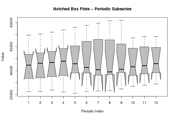
22577.0 22792.0 23932.0 22321.0 21102.0 22824.0 23129.0 23604.0 24746.0 26911.0 27909.0 28922.0 29800.0 30506.0 30771.0 31976.0 33749.0 34371.0 33246.0 35072.0 35762.0 36179.0 37433.0 38298.0 37559.0 37511.0 39364.0 40084.0 42712.0 41938.0 40799.0 38568.0 41134.0 43955.0 43607.0 45082.0 46464.0 46496.0 46774.0 47890.0 45740.0 42660.0 39190.0 39010.0 41150.0 42530.0 44710.0 46620.0 44560.0 46120.0 48060.0 51970.0 57720.0 63490.0 65370.0 64260.0 58700.0 58630.0 59803.0 59266.0 60570.0 63062.0 63846.0 64726.0 63460.0 65220.0 66659.0 66871.0 65672.0 67182.0 68292.0 68318.0 69530.0 70500.0 72044.0 73811.0 76018.0 77818.0 79455.0 81408.0 81815.0 | |||||||||||||||||||||
Tables (Output of Computation) | |||||||||||||||||||||
| |||||||||||||||||||||
Figures (Output of Computation) | |||||||||||||||||||||
Input Parameters & R Code | |||||||||||||||||||||
| Parameters (Session): | |||||||||||||||||||||
| par1 = 12 ; | |||||||||||||||||||||
| Parameters (R input): | |||||||||||||||||||||
| par1 = 12 ; | |||||||||||||||||||||
| R code (references can be found in the software module): | |||||||||||||||||||||
par1 <- as.numeric(par1) | |||||||||||||||||||||