Free Statistics
of Irreproducible Research!
Description of Statistical Computation | |||||||||||||||||||||
|---|---|---|---|---|---|---|---|---|---|---|---|---|---|---|---|---|---|---|---|---|---|
| Author's title | |||||||||||||||||||||
| Author | *Unverified author* | ||||||||||||||||||||
| R Software Module | rwasp_sdplot.wasp | ||||||||||||||||||||
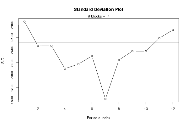
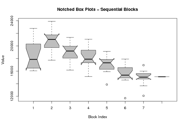
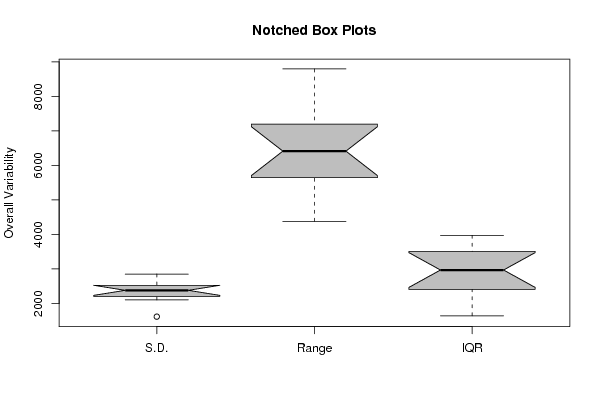
| Title produced by software | Standard Deviation Plot | ||||||||||||||||||||
| Date of computation | Sun, 16 May 2010 18:04:00 +0000 | ||||||||||||||||||||
| Cite this page as follows | Statistical Computations at FreeStatistics.org, Office for Research Development and Education, URL https://freestatistics.org/blog/index.php?v=date/2010/May/16/t1274033160wcc62o7dqv6jd77.htm/, Retrieved Mon, 29 Apr 2024 20:01:21 +0000 | ||||||||||||||||||||
| Statistical Computations at FreeStatistics.org, Office for Research Development and Education, URL https://freestatistics.org/blog/index.php?pk=76040, Retrieved Mon, 29 Apr 2024 20:01:21 +0000 | |||||||||||||||||||||
| QR Codes: | |||||||||||||||||||||
|
| |||||||||||||||||||||
| Original text written by user: | |||||||||||||||||||||
| IsPrivate? | No (this computation is public) | ||||||||||||||||||||
| User-defined keywords | KDGP2W83 | ||||||||||||||||||||
| Estimated Impact | 185 | ||||||||||||||||||||
Tree of Dependent Computations | |||||||||||||||||||||
| Family? (F = Feedback message, R = changed R code, M = changed R Module, P = changed Parameters, D = changed Data) | |||||||||||||||||||||
| - [Univariate Data Series] [Uitvoer van Belgi�] [2010-02-04 08:24:53] [2ee36997fb1be82ef07372b18c1a823d] - RMPD [Standard Deviation Plot] [invoer uitvoer be...] [2010-05-16 18:04:00] [ea4db07d8da34007b79212461ea6aa7b] [Current] | |||||||||||||||||||||
| Feedback Forum | |||||||||||||||||||||
Post a new message | |||||||||||||||||||||
Dataset | |||||||||||||||||||||
| Dataseries X: | |||||||||||||||||||||
18288.3 16049 16764.5 17880.2 16555.9 16087.1 16373.5 17842.2 22321.5 22786.7 18274.1 22392.9 23899.3 21343.5 22952.3 21374.4 21164.1 20906.5 17877.4 20664.3 22160 19813.6 17735.4 19640.2 20844.4 19823.1 18594.6 21350.6 18574.1 18924.2 17343.4 19961.2 19932.1 19464.6 16165.4 17574.9 19795.4 19439.5 17170 21072.4 17751.8 17515.5 18040.3 19090.1 17746.5 19202.1 15141.6 16258.1 18586.5 17209.4 17838.7 19123.5 16583.6 15991.2 16704.5 17422 17872 17823.2 13866.5 15912.8 17870.5 15420.3 16379.4 17903.9 15305.8 14583.3 14861 14968.9 16726.5 16283.6 11703.7 15101.8 15469.7 14956.9 15370.6 15998.1 14725.1 14768.9 13659.6 15070.3 16942.6 15761.3 12083 15023.6 15106.5 | |||||||||||||||||||||
Tables (Output of Computation) | |||||||||||||||||||||
| |||||||||||||||||||||
Figures (Output of Computation) | |||||||||||||||||||||
Input Parameters & R Code | |||||||||||||||||||||
| Parameters (Session): | |||||||||||||||||||||
| par1 = 12 ; | |||||||||||||||||||||
| Parameters (R input): | |||||||||||||||||||||
| par1 = 12 ; | |||||||||||||||||||||
| R code (references can be found in the software module): | |||||||||||||||||||||
par1 <- as.numeric(par1) | |||||||||||||||||||||