Free Statistics

of Irreproducible Research!

Author's title

Author*The author of this computation has been verified*
R Software Modulerwasp_pairs.wasp
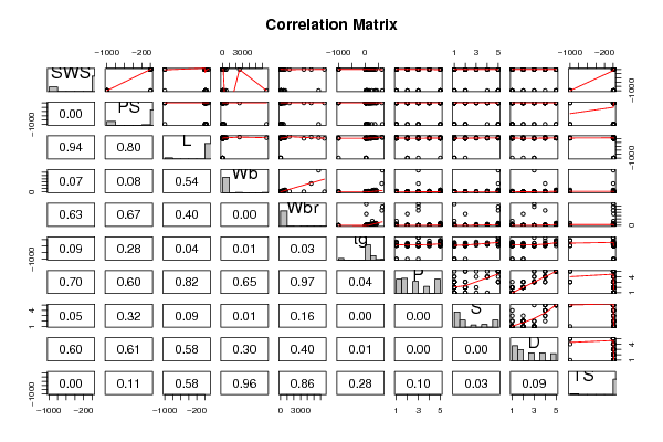
Title produced by softwareKendall tau Correlation Matrix
Date of computationTue, 21 Dec 2010 12:11:35 +0000
Cite this page as followsStatistical Computations at FreeStatistics.org, Office for Research Development and Education, URL https://freestatistics.org/blog/index.php?v=date/2010/Dec/21/t12929333972cwyd32x0o0nivp.htm/, Retrieved Fri, 17 May 2024 07:00:06 +0000
Statistical Computations at FreeStatistics.org, Office for Research Development and Education, URL https://freestatistics.org/blog/index.php?pk=113351, Retrieved Fri, 17 May 2024 07:00:06 +0000
QR Codes:

Original text written by user:
IsPrivate?No (this computation is public)
User-defined keywords
Estimated Impact150
Family? (F = Feedback message, R = changed R code, M = changed R Module, P = changed Parameters, D = changed Data)
-       [Kendall tau Correlation Matrix] [] [2010-12-21 12:11:35] [9d4f9c24554023ef0148ede5dd3a4d11] [Current]
Feedback Forum

Post a new message
Dataseries X:
-999,000	-999,000	38,600	6654,000	5712,000	645,000	3,000	5,000	3,000	3,300
6,300	2,000	4,500	1,000	6600,000	42,000	3,000	1,000	3,000	8,300
-999,000	-999,000	14,000	3,385	44,500	60,000	1,000	1,000	1,000	12,500
-999,000	-999,000	-999,000	0,920	5,700	25,000	5,000	2,000	3,000	16,500
2,100	1,800	69,000	2547,000	4603,000	624,000	3,000	5,000	4,000	3,900
9,100	0,700	27,000	10,550	179,500	180,000	4,000	4,000	4,000	9,800
15,800	3,900	19,000	0,023	0,300	35,000	1,000	1,000	1,000	19,700
5,200	1,000	30,400	160,000	169,000	392,000	4,000	5,000	4,000	6,200
10,900	3,600	28,000	3,300	25,600	63,000	1,000	2,000	1,000	14,500
8,300	1,400	50,000	52,160	440,000	230,000	1,000	1,000	1,000	9,700
11,000	1,500	7,000	0,425	6,400	112,000	5,000	4,000	4,000	12,500
3,200	0,700	30,000	465,000	423,000	281,000	5,000	5,000	5,000	3,900
7,600	2,700	-999,000	0,550	2,400	-999,000	2,000	1,000	2,000	10,300
-999,000	-999,000	40,000	187,100	419,000	365,000	5,000	5,000	5,000	3,100
6,300	2,100	3,500	0,075	1,200	42,000	1,000	1,000	1,000	8,400
8,600	0,000	50,000	3,000	25,000	28,000	2,000	2,000	2,000	8,600
6,600	4,100	6,000	0,785	3500,000	42,000	2,000	2,000	2,000	10,700
9,500	1,200	10,400	0,200	5,000	120,000	2,000	2,000	2,000	10,700
4,800	1,300	34,000	1,410	17,500	-999,000	1,000	2,000	1,000	6,100
12,000	6,100	7,000	60,000	81,000	-999,000	1,000	1,000	1,000	18,100
-999,000	0,300	28,000	529,000	680,000	400,000	5,000	5,000	5,000	-999,000
3,300	0,500	20,000	27,660	115,000	148,000	5,000	5,000	5,000	3,800
11,000	3,400	3,900	0,120	1,000	16,000	3,000	1,000	2,000	14,400
-999,000	-999,000	39,300	207,000	406,000	252,000	1,000	4,000	1,000	12,000
4,700	1,500	41,000	85,000	325,000	310,000	1,000	3,000	1,000	6,200
-999,000	-999,000	16,200	36,330	119,500	63,000	1,000	1,000	1,000	13,000
10,400	3,400	9,000	0,101	4,000	28,000	5,000	1,000	3,000	13,800
7,400	0,800	7,600	1,040	5,500	68,000	5,000	3,000	4,000	8,200
2,100	0,800	46,000	521,000	655,000	336,000	5,000	5,000	5,000	2,900
-999,000	-999,000	22,400	100,000	157,000	100,000	1,000	1,000	1,000	10,800
-999,000	-999,000	16,300	35,000	56,000	33,000	3,000	5,000	4,000	-999,000
7,700	1,400	2,600	0,005	0,140	21,500	5,000	2,000	4,000	9,100
17,900	2,000	24,000	0,010	0,250	50,000	1,000	1,000	1,000	19,900
6,100	1,900	100,000	62,000	1320,000	267,000	1,000	1,000	1,000	8,000
8,200	2,400	-999,000	0,122	3,000	30,000	2,000	1,000	1,000	10,600
8,400	2,800	-999,000	1,350	8,100	45,000	3,000	1,000	3,000	11,200
11,900	1,300	3,200	0,023	0,400	19,000	4,000	1,000	3,000	13,200
10,800	2,000	2,000	0,048	0,330	30,000	4,000	1,000	3,000	12,800
13,800	5,600	5,000	1,700	6,300	12,000	2,000	1,000	1,000	19,400
14,300	3,100	6,500	3,500	10,800	120,000	2,000	1,000	1,000	17,400
-999,000	1,000	23,600	250,000	490,000	440,000	5,000	5,000	5,000	-999,000
15,200	1,800	12,000	0,480	15,500	140,000	2,000	2,000	2,000	17,000
10,000	0,900	20,200	10,000	115,000	170,000	4,000	4,000	4,000	10,900
11,900	1,800	13,000	1,620	11,400	17,000	2,000	1,000	2,000	13,700
6,500	1,900	27,000	192,000	180,000	115,000	4,000	4,000	4,000	8,400
7,500	0,900	18,000	2,500	12,100	31,000	5,000	5,000	5,000	8,400
-999,000	-999,000	13,700	4,288	39,200	63,000	2,000	2,000	2,000	12,500
10,600	2,600	4,700	0,280	1,900	21,000	3,000	1,000	3,000	13,200
7,400	2,400	9,800	4,235	50,400	52,000	1,000	1,000	1,000	9,800
8,400	1,200	29,000	6,800	179,000	164,000	2,000	3,000	2,000	9,600
5,700	0,900	7,000	0,750	12,300	225,000	2,000	2,000	2,000	6,600
4,900	0,500	6,000	3,600	21,000	225,000	3,000	2,000	3,000	5,400
-999,000	-999,000	17,000	14,830	98,200	150,000	5,000	5,000	5,000	2,600
3,200	0,600	20,000	55,500	175,000	151,000	5,000	5,000	5,000	3,800
-999,000	-999,000	12,700	1,400	12,500	90,000	2,000	2,000	2,000	11,000
8,100	2,200	3,500	0,060	1,000	-999,000	3,000	1,000	2,000	10,300
11,000	2,300	4,500	0,900	2,600	60,000	2,000	1,000	2,000	13,300
4,900	0,500	7,500	2,000	12,300	200,000	3,000	1,000	3,000	5,400
13,200	2,600	2,300	0,104	2,500	46,000	3,000	2,000	2,000	15,800
9,700	0,600	24,000	4,190	58,000	210,000	4,000	3,000	4,000	10,300
12,800	6,600	3,000	3,500	3,900	14,000	2,000	1,000	1,000	19,400
-999,000	-999,000	13,000	4,050	17,000	38,000	3,000	1,000	1,000	-999,000


Summary of computational transaction
Raw Inputview raw input (R code)
Raw Outputview raw output of R engine
Computing time3 seconds
R Server'George Udny Yule' @ 72.249.76.132
R Framework error message
The field 'Names of X columns' contains a hard return which cannot be interpreted.
Please, resubmit your request without hard returns in the 'Names of X columns'.

\begin{tabular}{lllllllll}
\hline
Summary of computational transaction \tabularnewline
Raw Input & view raw input (R code)  \tabularnewline
Raw Output & view raw output of R engine  \tabularnewline
Computing time & 3 seconds \tabularnewline
R Server & 'George Udny Yule' @ 72.249.76.132 \tabularnewline
R Framework error message & 
The field 'Names of X columns' contains a hard return which cannot be interpreted.
Please, resubmit your request without hard returns in the 'Names of X columns'.
\tabularnewline \hline \end{tabular} %Source: https://freestatistics.org/blog/index.php?pk=113351&T=0

[TABLE]
[ROW][C]Summary of computational transaction[/C][/ROW]
[ROW][C]Raw Input[/C][C]view raw input (R code) [/C][/ROW]
[ROW][C]Raw Output[/C][C]view raw output of R engine [/C][/ROW]
[ROW][C]Computing time[/C][C]3 seconds[/C][/ROW]
[ROW][C]R Server[/C][C]'George Udny Yule' @ 72.249.76.132[/C][/ROW]
[ROW][C]R Framework error message[/C][C]
The field 'Names of X columns' contains a hard return which cannot be interpreted.
Please, resubmit your request without hard returns in the 'Names of X columns'.
[/C][/ROW] [/TABLE] Source: https://freestatistics.org/blog/index.php?pk=113351&T=0

Globally Unique Identifier (entire table): ba.freestatistics.org/blog/index.php?pk=113351&T=0

As an alternative you can also use a QR Code:  

The GUIDs for individual cells are displayed in the table below:

Summary of computational transaction
Raw Inputview raw input (R code)
Raw Outputview raw output of R engine
Computing time3 seconds
R Server'George Udny Yule' @ 72.249.76.132
R Framework error message
The field 'Names of X columns' contains a hard return which cannot be interpreted.
Please, resubmit your request without hard returns in the 'Names of X columns'.


Correlations for all pairs of data series (method=pearson)
SWSPSLWbWbrtgPSDTS
SWS10.9070.01-0.228-0.063-0.218-0.05-0.249-0.0680.488
PS0.90710.033-0.223-0.055-0.1390.067-0.1290.0660.205
L0.010.03310.0790.1080.267-0.030.2170.071-0.071
Wb-0.228-0.2230.07910.6460.340.0590.3380.134-0.007
Wbr-0.063-0.0550.1080.64610.2780.0060.180.1090.022
tg-0.218-0.1390.2670.340.27810.2670.4530.348-0.138
P-0.050.067-0.030.0590.0060.26710.6180.916-0.209
S-0.249-0.1290.2170.3380.180.4530.61810.787-0.271
D-0.0680.0660.0710.1340.1090.3480.9160.7871-0.219
TS 0.4880.205-0.071-0.0070.022-0.138-0.209-0.271-0.2191

\begin{tabular}{lllllllll}
\hline
Correlations for all pairs of data series (method=pearson) \tabularnewline
  & SWS & PS & L & Wb & Wbr & tg & P & S & D & TS
 \tabularnewline
SWS & 1 & 0.907 & 0.01 & -0.228 & -0.063 & -0.218 & -0.05 & -0.249 & -0.068 & 0.488 \tabularnewline
PS & 0.907 & 1 & 0.033 & -0.223 & -0.055 & -0.139 & 0.067 & -0.129 & 0.066 & 0.205 \tabularnewline
L & 0.01 & 0.033 & 1 & 0.079 & 0.108 & 0.267 & -0.03 & 0.217 & 0.071 & -0.071 \tabularnewline
Wb & -0.228 & -0.223 & 0.079 & 1 & 0.646 & 0.34 & 0.059 & 0.338 & 0.134 & -0.007 \tabularnewline
Wbr & -0.063 & -0.055 & 0.108 & 0.646 & 1 & 0.278 & 0.006 & 0.18 & 0.109 & 0.022 \tabularnewline
tg & -0.218 & -0.139 & 0.267 & 0.34 & 0.278 & 1 & 0.267 & 0.453 & 0.348 & -0.138 \tabularnewline
P & -0.05 & 0.067 & -0.03 & 0.059 & 0.006 & 0.267 & 1 & 0.618 & 0.916 & -0.209 \tabularnewline
S & -0.249 & -0.129 & 0.217 & 0.338 & 0.18 & 0.453 & 0.618 & 1 & 0.787 & -0.271 \tabularnewline
D & -0.068 & 0.066 & 0.071 & 0.134 & 0.109 & 0.348 & 0.916 & 0.787 & 1 & -0.219 \tabularnewline
TS
 & 0.488 & 0.205 & -0.071 & -0.007 & 0.022 & -0.138 & -0.209 & -0.271 & -0.219 & 1 \tabularnewline
\hline
\end{tabular}
%Source: https://freestatistics.org/blog/index.php?pk=113351&T=1

[TABLE]
[ROW][C]Correlations for all pairs of data series (method=pearson)[/C][/ROW]
[ROW][C] [/C][C]SWS[/C][C]PS[/C][C]L[/C][C]Wb[/C][C]Wbr[/C][C]tg[/C][C]P[/C][C]S[/C][C]D[/C][C]TS
[/C][/ROW]
[ROW][C]SWS[/C][C]1[/C][C]0.907[/C][C]0.01[/C][C]-0.228[/C][C]-0.063[/C][C]-0.218[/C][C]-0.05[/C][C]-0.249[/C][C]-0.068[/C][C]0.488[/C][/ROW]
[ROW][C]PS[/C][C]0.907[/C][C]1[/C][C]0.033[/C][C]-0.223[/C][C]-0.055[/C][C]-0.139[/C][C]0.067[/C][C]-0.129[/C][C]0.066[/C][C]0.205[/C][/ROW]
[ROW][C]L[/C][C]0.01[/C][C]0.033[/C][C]1[/C][C]0.079[/C][C]0.108[/C][C]0.267[/C][C]-0.03[/C][C]0.217[/C][C]0.071[/C][C]-0.071[/C][/ROW]
[ROW][C]Wb[/C][C]-0.228[/C][C]-0.223[/C][C]0.079[/C][C]1[/C][C]0.646[/C][C]0.34[/C][C]0.059[/C][C]0.338[/C][C]0.134[/C][C]-0.007[/C][/ROW]
[ROW][C]Wbr[/C][C]-0.063[/C][C]-0.055[/C][C]0.108[/C][C]0.646[/C][C]1[/C][C]0.278[/C][C]0.006[/C][C]0.18[/C][C]0.109[/C][C]0.022[/C][/ROW]
[ROW][C]tg[/C][C]-0.218[/C][C]-0.139[/C][C]0.267[/C][C]0.34[/C][C]0.278[/C][C]1[/C][C]0.267[/C][C]0.453[/C][C]0.348[/C][C]-0.138[/C][/ROW]
[ROW][C]P[/C][C]-0.05[/C][C]0.067[/C][C]-0.03[/C][C]0.059[/C][C]0.006[/C][C]0.267[/C][C]1[/C][C]0.618[/C][C]0.916[/C][C]-0.209[/C][/ROW]
[ROW][C]S[/C][C]-0.249[/C][C]-0.129[/C][C]0.217[/C][C]0.338[/C][C]0.18[/C][C]0.453[/C][C]0.618[/C][C]1[/C][C]0.787[/C][C]-0.271[/C][/ROW]
[ROW][C]D[/C][C]-0.068[/C][C]0.066[/C][C]0.071[/C][C]0.134[/C][C]0.109[/C][C]0.348[/C][C]0.916[/C][C]0.787[/C][C]1[/C][C]-0.219[/C][/ROW]
[ROW][C]TS
[/C][C]0.488[/C][C]0.205[/C][C]-0.071[/C][C]-0.007[/C][C]0.022[/C][C]-0.138[/C][C]-0.209[/C][C]-0.271[/C][C]-0.219[/C][C]1[/C][/ROW]
[/TABLE]
Source: https://freestatistics.org/blog/index.php?pk=113351&T=1

Globally Unique Identifier (entire table): ba.freestatistics.org/blog/index.php?pk=113351&T=1

As an alternative you can also use a QR Code:  

The GUIDs for individual cells are displayed in the table below:

Correlations for all pairs of data series (method=pearson)
SWSPSLWbWbrtgPSDTS
SWS10.9070.01-0.228-0.063-0.218-0.05-0.249-0.0680.488
PS0.90710.033-0.223-0.055-0.1390.067-0.1290.0660.205
L0.010.03310.0790.1080.267-0.030.2170.071-0.071
Wb-0.228-0.2230.07910.6460.340.0590.3380.134-0.007
Wbr-0.063-0.0550.1080.64610.2780.0060.180.1090.022
tg-0.218-0.1390.2670.340.27810.2670.4530.348-0.138
P-0.050.067-0.030.0590.0060.26710.6180.916-0.209
S-0.249-0.1290.2170.3380.180.4530.61810.787-0.271
D-0.0680.0660.0710.1340.1090.3480.9160.7871-0.219
TS 0.4880.205-0.071-0.0070.022-0.138-0.209-0.271-0.2191


Correlations for all pairs of data series with p-values
pairPearson rSpearman rhoKendall tau
SWS;PS0.90740.76680.5954
p-value(0)(0)(0)
SWS;L0.0097-0.3691-0.2469
p-value(0.9406)(0.0032)(0.0057)
SWS;Wb-0.2279-0.5942-0.422
p-value(0.0749)(0)(0)
SWS;Wbr-0.0628-0.5783-0.402
p-value(0.6277)(0)(0)
SWS;tg-0.2178-0.4493-0.3271
p-value(0.089)(2e-04)(2e-04)
SWS;P-0.0496-0.1722-0.1359
p-value(0.7017)(0.1808)(0.1603)
SWS;S-0.2488-0.4595-0.363
p-value(0.0512)(2e-04)(2e-04)
SWS;D-0.0683-0.2668-0.2189
p-value(0.5977)(0.036)(0.024)
SWS;TS 0.48750.70540.636
p-value(1e-04)(0)(0)
PS;L0.033-0.4284-0.2684
p-value(0.7987)(5e-04)(0.0026)
PS;Wb-0.2227-0.4751-0.3085
p-value(0.0819)(1e-04)(5e-04)
PS;Wbr-0.0554-0.4082-0.2527
p-value(0.669)(0.001)(0.0045)
PS;tg-0.139-0.4703-0.3228
p-value(0.2813)(1e-04)(3e-04)
PS;P0.0671-0.2648-0.2039
p-value(0.6045)(0.0375)(0.035)
PS;S-0.1289-0.5117-0.4007
p-value(0.318)(0)(0)
PS;D0.0656-0.3525-0.2826
p-value(0.6125)(0.005)(0.0035)
PS;TS 0.20550.54130.4193
p-value(0.1091)(0)(0)
L;Wb0.07920.72690.5407
p-value(0.5407)(0)(0)
L;Wbr0.10840.71260.5669
p-value(0.4017)(0)(0)
L;tg0.26720.65440.4772
p-value(0.0358)(0)(0)
L;P-0.0301-0.0651-0.0593
p-value(0.8166)(0.6149)(0.5332)
L;S0.2170.55090.4154
p-value(0.0903)(0)(0)
L;D0.07070.13160.0894
p-value(0.5848)(0.308)(0.3484)
L;TS -0.0714-0.4571-0.3021
p-value(0.5815)(2e-04)(6e-04)
Wb;Wbr0.64630.86750.7583
p-value(0)(0)(0)
Wb;tg0.33990.68120.5081
p-value(0.0069)(0)(0)
Wb;P0.05950.09380.0591
p-value(0.646)(0.4684)(0.5333)
Wb;S0.33830.57110.4554
p-value(0.0072)(0)(0)
Wb;D0.13360.2510.1721
p-value(0.3006)(0.0491)(0.07)
Wb;TS -0.0071-0.5531-0.3844
p-value(0.956)(0)(0)
Wbr;tg0.27790.69670.5183
p-value(0.0288)(0)(0)
Wbr;P0.00550.05950.0313
p-value(0.966)(0.6461)(0.7413)
Wbr;S0.17980.54910.443
p-value(0.1621)(0)(0)
Wbr;D0.1090.25070.1727
p-value(0.3993)(0.0493)(0.069)
Wbr;TS 0.0225-0.5748-0.3956
p-value(0.8625)(0)(0)
tg;P0.26680.18980.1299
p-value(0.0361)(0.1395)(0.1724)
tg;S0.45270.6190.499
p-value(2e-04)(0)(0)
tg;D0.34830.36110.264
p-value(0.0055)(0.0039)(0.0056)
tg;TS -0.1382-0.5426-0.3987
p-value(0.284)(0)(0)
P;S0.61820.56690.4693
p-value(0)(0)(0)
P;D0.9160.9180.8563
p-value(0)(0)(0)
P;TS -0.2092-0.4035-0.3053
p-value(0.1027)(0.0011)(0.0014)
S;D0.78720.71810.6277
p-value(0)(0)(0)
S;TS -0.2713-0.6111-0.4867
p-value(0.0329)(0)(0)
D;TS -0.2186-0.5283-0.4184
p-value(0.0878)(0)(0)

\begin{tabular}{lllllllll}
\hline
Correlations for all pairs of data series with p-values \tabularnewline
pair & Pearson r & Spearman rho & Kendall tau \tabularnewline
SWS;PS & 0.9074 & 0.7668 & 0.5954 \tabularnewline
p-value & (0) & (0) & (0) \tabularnewline
SWS;L & 0.0097 & -0.3691 & -0.2469 \tabularnewline
p-value & (0.9406) & (0.0032) & (0.0057) \tabularnewline
SWS;Wb & -0.2279 & -0.5942 & -0.422 \tabularnewline
p-value & (0.0749) & (0) & (0) \tabularnewline
SWS;Wbr & -0.0628 & -0.5783 & -0.402 \tabularnewline
p-value & (0.6277) & (0) & (0) \tabularnewline
SWS;tg & -0.2178 & -0.4493 & -0.3271 \tabularnewline
p-value & (0.089) & (2e-04) & (2e-04) \tabularnewline
SWS;P & -0.0496 & -0.1722 & -0.1359 \tabularnewline
p-value & (0.7017) & (0.1808) & (0.1603) \tabularnewline
SWS;S & -0.2488 & -0.4595 & -0.363 \tabularnewline
p-value & (0.0512) & (2e-04) & (2e-04) \tabularnewline
SWS;D & -0.0683 & -0.2668 & -0.2189 \tabularnewline
p-value & (0.5977) & (0.036) & (0.024) \tabularnewline
SWS;TS
 & 0.4875 & 0.7054 & 0.636 \tabularnewline
p-value & (1e-04) & (0) & (0) \tabularnewline
PS;L & 0.033 & -0.4284 & -0.2684 \tabularnewline
p-value & (0.7987) & (5e-04) & (0.0026) \tabularnewline
PS;Wb & -0.2227 & -0.4751 & -0.3085 \tabularnewline
p-value & (0.0819) & (1e-04) & (5e-04) \tabularnewline
PS;Wbr & -0.0554 & -0.4082 & -0.2527 \tabularnewline
p-value & (0.669) & (0.001) & (0.0045) \tabularnewline
PS;tg & -0.139 & -0.4703 & -0.3228 \tabularnewline
p-value & (0.2813) & (1e-04) & (3e-04) \tabularnewline
PS;P & 0.0671 & -0.2648 & -0.2039 \tabularnewline
p-value & (0.6045) & (0.0375) & (0.035) \tabularnewline
PS;S & -0.1289 & -0.5117 & -0.4007 \tabularnewline
p-value & (0.318) & (0) & (0) \tabularnewline
PS;D & 0.0656 & -0.3525 & -0.2826 \tabularnewline
p-value & (0.6125) & (0.005) & (0.0035) \tabularnewline
PS;TS
 & 0.2055 & 0.5413 & 0.4193 \tabularnewline
p-value & (0.1091) & (0) & (0) \tabularnewline
L;Wb & 0.0792 & 0.7269 & 0.5407 \tabularnewline
p-value & (0.5407) & (0) & (0) \tabularnewline
L;Wbr & 0.1084 & 0.7126 & 0.5669 \tabularnewline
p-value & (0.4017) & (0) & (0) \tabularnewline
L;tg & 0.2672 & 0.6544 & 0.4772 \tabularnewline
p-value & (0.0358) & (0) & (0) \tabularnewline
L;P & -0.0301 & -0.0651 & -0.0593 \tabularnewline
p-value & (0.8166) & (0.6149) & (0.5332) \tabularnewline
L;S & 0.217 & 0.5509 & 0.4154 \tabularnewline
p-value & (0.0903) & (0) & (0) \tabularnewline
L;D & 0.0707 & 0.1316 & 0.0894 \tabularnewline
p-value & (0.5848) & (0.308) & (0.3484) \tabularnewline
L;TS
 & -0.0714 & -0.4571 & -0.3021 \tabularnewline
p-value & (0.5815) & (2e-04) & (6e-04) \tabularnewline
Wb;Wbr & 0.6463 & 0.8675 & 0.7583 \tabularnewline
p-value & (0) & (0) & (0) \tabularnewline
Wb;tg & 0.3399 & 0.6812 & 0.5081 \tabularnewline
p-value & (0.0069) & (0) & (0) \tabularnewline
Wb;P & 0.0595 & 0.0938 & 0.0591 \tabularnewline
p-value & (0.646) & (0.4684) & (0.5333) \tabularnewline
Wb;S & 0.3383 & 0.5711 & 0.4554 \tabularnewline
p-value & (0.0072) & (0) & (0) \tabularnewline
Wb;D & 0.1336 & 0.251 & 0.1721 \tabularnewline
p-value & (0.3006) & (0.0491) & (0.07) \tabularnewline
Wb;TS
 & -0.0071 & -0.5531 & -0.3844 \tabularnewline
p-value & (0.956) & (0) & (0) \tabularnewline
Wbr;tg & 0.2779 & 0.6967 & 0.5183 \tabularnewline
p-value & (0.0288) & (0) & (0) \tabularnewline
Wbr;P & 0.0055 & 0.0595 & 0.0313 \tabularnewline
p-value & (0.966) & (0.6461) & (0.7413) \tabularnewline
Wbr;S & 0.1798 & 0.5491 & 0.443 \tabularnewline
p-value & (0.1621) & (0) & (0) \tabularnewline
Wbr;D & 0.109 & 0.2507 & 0.1727 \tabularnewline
p-value & (0.3993) & (0.0493) & (0.069) \tabularnewline
Wbr;TS
 & 0.0225 & -0.5748 & -0.3956 \tabularnewline
p-value & (0.8625) & (0) & (0) \tabularnewline
tg;P & 0.2668 & 0.1898 & 0.1299 \tabularnewline
p-value & (0.0361) & (0.1395) & (0.1724) \tabularnewline
tg;S & 0.4527 & 0.619 & 0.499 \tabularnewline
p-value & (2e-04) & (0) & (0) \tabularnewline
tg;D & 0.3483 & 0.3611 & 0.264 \tabularnewline
p-value & (0.0055) & (0.0039) & (0.0056) \tabularnewline
tg;TS
 & -0.1382 & -0.5426 & -0.3987 \tabularnewline
p-value & (0.284) & (0) & (0) \tabularnewline
P;S & 0.6182 & 0.5669 & 0.4693 \tabularnewline
p-value & (0) & (0) & (0) \tabularnewline
P;D & 0.916 & 0.918 & 0.8563 \tabularnewline
p-value & (0) & (0) & (0) \tabularnewline
P;TS
 & -0.2092 & -0.4035 & -0.3053 \tabularnewline
p-value & (0.1027) & (0.0011) & (0.0014) \tabularnewline
S;D & 0.7872 & 0.7181 & 0.6277 \tabularnewline
p-value & (0) & (0) & (0) \tabularnewline
S;TS
 & -0.2713 & -0.6111 & -0.4867 \tabularnewline
p-value & (0.0329) & (0) & (0) \tabularnewline
D;TS
 & -0.2186 & -0.5283 & -0.4184 \tabularnewline
p-value & (0.0878) & (0) & (0) \tabularnewline
\hline
\end{tabular}
%Source: https://freestatistics.org/blog/index.php?pk=113351&T=2

[TABLE]
[ROW][C]Correlations for all pairs of data series with p-values[/C][/ROW]
[ROW][C]pair[/C][C]Pearson r[/C][C]Spearman rho[/C][C]Kendall tau[/C][/ROW]
[ROW][C]SWS;PS[/C][C]0.9074[/C][C]0.7668[/C][C]0.5954[/C][/ROW]
[ROW][C]p-value[/C][C](0)[/C][C](0)[/C][C](0)[/C][/ROW]
[ROW][C]SWS;L[/C][C]0.0097[/C][C]-0.3691[/C][C]-0.2469[/C][/ROW]
[ROW][C]p-value[/C][C](0.9406)[/C][C](0.0032)[/C][C](0.0057)[/C][/ROW]
[ROW][C]SWS;Wb[/C][C]-0.2279[/C][C]-0.5942[/C][C]-0.422[/C][/ROW]
[ROW][C]p-value[/C][C](0.0749)[/C][C](0)[/C][C](0)[/C][/ROW]
[ROW][C]SWS;Wbr[/C][C]-0.0628[/C][C]-0.5783[/C][C]-0.402[/C][/ROW]
[ROW][C]p-value[/C][C](0.6277)[/C][C](0)[/C][C](0)[/C][/ROW]
[ROW][C]SWS;tg[/C][C]-0.2178[/C][C]-0.4493[/C][C]-0.3271[/C][/ROW]
[ROW][C]p-value[/C][C](0.089)[/C][C](2e-04)[/C][C](2e-04)[/C][/ROW]
[ROW][C]SWS;P[/C][C]-0.0496[/C][C]-0.1722[/C][C]-0.1359[/C][/ROW]
[ROW][C]p-value[/C][C](0.7017)[/C][C](0.1808)[/C][C](0.1603)[/C][/ROW]
[ROW][C]SWS;S[/C][C]-0.2488[/C][C]-0.4595[/C][C]-0.363[/C][/ROW]
[ROW][C]p-value[/C][C](0.0512)[/C][C](2e-04)[/C][C](2e-04)[/C][/ROW]
[ROW][C]SWS;D[/C][C]-0.0683[/C][C]-0.2668[/C][C]-0.2189[/C][/ROW]
[ROW][C]p-value[/C][C](0.5977)[/C][C](0.036)[/C][C](0.024)[/C][/ROW]
[ROW][C]SWS;TS
[/C][C]0.4875[/C][C]0.7054[/C][C]0.636[/C][/ROW]
[ROW][C]p-value[/C][C](1e-04)[/C][C](0)[/C][C](0)[/C][/ROW]
[ROW][C]PS;L[/C][C]0.033[/C][C]-0.4284[/C][C]-0.2684[/C][/ROW]
[ROW][C]p-value[/C][C](0.7987)[/C][C](5e-04)[/C][C](0.0026)[/C][/ROW]
[ROW][C]PS;Wb[/C][C]-0.2227[/C][C]-0.4751[/C][C]-0.3085[/C][/ROW]
[ROW][C]p-value[/C][C](0.0819)[/C][C](1e-04)[/C][C](5e-04)[/C][/ROW]
[ROW][C]PS;Wbr[/C][C]-0.0554[/C][C]-0.4082[/C][C]-0.2527[/C][/ROW]
[ROW][C]p-value[/C][C](0.669)[/C][C](0.001)[/C][C](0.0045)[/C][/ROW]
[ROW][C]PS;tg[/C][C]-0.139[/C][C]-0.4703[/C][C]-0.3228[/C][/ROW]
[ROW][C]p-value[/C][C](0.2813)[/C][C](1e-04)[/C][C](3e-04)[/C][/ROW]
[ROW][C]PS;P[/C][C]0.0671[/C][C]-0.2648[/C][C]-0.2039[/C][/ROW]
[ROW][C]p-value[/C][C](0.6045)[/C][C](0.0375)[/C][C](0.035)[/C][/ROW]
[ROW][C]PS;S[/C][C]-0.1289[/C][C]-0.5117[/C][C]-0.4007[/C][/ROW]
[ROW][C]p-value[/C][C](0.318)[/C][C](0)[/C][C](0)[/C][/ROW]
[ROW][C]PS;D[/C][C]0.0656[/C][C]-0.3525[/C][C]-0.2826[/C][/ROW]
[ROW][C]p-value[/C][C](0.6125)[/C][C](0.005)[/C][C](0.0035)[/C][/ROW]
[ROW][C]PS;TS
[/C][C]0.2055[/C][C]0.5413[/C][C]0.4193[/C][/ROW]
[ROW][C]p-value[/C][C](0.1091)[/C][C](0)[/C][C](0)[/C][/ROW]
[ROW][C]L;Wb[/C][C]0.0792[/C][C]0.7269[/C][C]0.5407[/C][/ROW]
[ROW][C]p-value[/C][C](0.5407)[/C][C](0)[/C][C](0)[/C][/ROW]
[ROW][C]L;Wbr[/C][C]0.1084[/C][C]0.7126[/C][C]0.5669[/C][/ROW]
[ROW][C]p-value[/C][C](0.4017)[/C][C](0)[/C][C](0)[/C][/ROW]
[ROW][C]L;tg[/C][C]0.2672[/C][C]0.6544[/C][C]0.4772[/C][/ROW]
[ROW][C]p-value[/C][C](0.0358)[/C][C](0)[/C][C](0)[/C][/ROW]
[ROW][C]L;P[/C][C]-0.0301[/C][C]-0.0651[/C][C]-0.0593[/C][/ROW]
[ROW][C]p-value[/C][C](0.8166)[/C][C](0.6149)[/C][C](0.5332)[/C][/ROW]
[ROW][C]L;S[/C][C]0.217[/C][C]0.5509[/C][C]0.4154[/C][/ROW]
[ROW][C]p-value[/C][C](0.0903)[/C][C](0)[/C][C](0)[/C][/ROW]
[ROW][C]L;D[/C][C]0.0707[/C][C]0.1316[/C][C]0.0894[/C][/ROW]
[ROW][C]p-value[/C][C](0.5848)[/C][C](0.308)[/C][C](0.3484)[/C][/ROW]
[ROW][C]L;TS
[/C][C]-0.0714[/C][C]-0.4571[/C][C]-0.3021[/C][/ROW]
[ROW][C]p-value[/C][C](0.5815)[/C][C](2e-04)[/C][C](6e-04)[/C][/ROW]
[ROW][C]Wb;Wbr[/C][C]0.6463[/C][C]0.8675[/C][C]0.7583[/C][/ROW]
[ROW][C]p-value[/C][C](0)[/C][C](0)[/C][C](0)[/C][/ROW]
[ROW][C]Wb;tg[/C][C]0.3399[/C][C]0.6812[/C][C]0.5081[/C][/ROW]
[ROW][C]p-value[/C][C](0.0069)[/C][C](0)[/C][C](0)[/C][/ROW]
[ROW][C]Wb;P[/C][C]0.0595[/C][C]0.0938[/C][C]0.0591[/C][/ROW]
[ROW][C]p-value[/C][C](0.646)[/C][C](0.4684)[/C][C](0.5333)[/C][/ROW]
[ROW][C]Wb;S[/C][C]0.3383[/C][C]0.5711[/C][C]0.4554[/C][/ROW]
[ROW][C]p-value[/C][C](0.0072)[/C][C](0)[/C][C](0)[/C][/ROW]
[ROW][C]Wb;D[/C][C]0.1336[/C][C]0.251[/C][C]0.1721[/C][/ROW]
[ROW][C]p-value[/C][C](0.3006)[/C][C](0.0491)[/C][C](0.07)[/C][/ROW]
[ROW][C]Wb;TS
[/C][C]-0.0071[/C][C]-0.5531[/C][C]-0.3844[/C][/ROW]
[ROW][C]p-value[/C][C](0.956)[/C][C](0)[/C][C](0)[/C][/ROW]
[ROW][C]Wbr;tg[/C][C]0.2779[/C][C]0.6967[/C][C]0.5183[/C][/ROW]
[ROW][C]p-value[/C][C](0.0288)[/C][C](0)[/C][C](0)[/C][/ROW]
[ROW][C]Wbr;P[/C][C]0.0055[/C][C]0.0595[/C][C]0.0313[/C][/ROW]
[ROW][C]p-value[/C][C](0.966)[/C][C](0.6461)[/C][C](0.7413)[/C][/ROW]
[ROW][C]Wbr;S[/C][C]0.1798[/C][C]0.5491[/C][C]0.443[/C][/ROW]
[ROW][C]p-value[/C][C](0.1621)[/C][C](0)[/C][C](0)[/C][/ROW]
[ROW][C]Wbr;D[/C][C]0.109[/C][C]0.2507[/C][C]0.1727[/C][/ROW]
[ROW][C]p-value[/C][C](0.3993)[/C][C](0.0493)[/C][C](0.069)[/C][/ROW]
[ROW][C]Wbr;TS
[/C][C]0.0225[/C][C]-0.5748[/C][C]-0.3956[/C][/ROW]
[ROW][C]p-value[/C][C](0.8625)[/C][C](0)[/C][C](0)[/C][/ROW]
[ROW][C]tg;P[/C][C]0.2668[/C][C]0.1898[/C][C]0.1299[/C][/ROW]
[ROW][C]p-value[/C][C](0.0361)[/C][C](0.1395)[/C][C](0.1724)[/C][/ROW]
[ROW][C]tg;S[/C][C]0.4527[/C][C]0.619[/C][C]0.499[/C][/ROW]
[ROW][C]p-value[/C][C](2e-04)[/C][C](0)[/C][C](0)[/C][/ROW]
[ROW][C]tg;D[/C][C]0.3483[/C][C]0.3611[/C][C]0.264[/C][/ROW]
[ROW][C]p-value[/C][C](0.0055)[/C][C](0.0039)[/C][C](0.0056)[/C][/ROW]
[ROW][C]tg;TS
[/C][C]-0.1382[/C][C]-0.5426[/C][C]-0.3987[/C][/ROW]
[ROW][C]p-value[/C][C](0.284)[/C][C](0)[/C][C](0)[/C][/ROW]
[ROW][C]P;S[/C][C]0.6182[/C][C]0.5669[/C][C]0.4693[/C][/ROW]
[ROW][C]p-value[/C][C](0)[/C][C](0)[/C][C](0)[/C][/ROW]
[ROW][C]P;D[/C][C]0.916[/C][C]0.918[/C][C]0.8563[/C][/ROW]
[ROW][C]p-value[/C][C](0)[/C][C](0)[/C][C](0)[/C][/ROW]
[ROW][C]P;TS
[/C][C]-0.2092[/C][C]-0.4035[/C][C]-0.3053[/C][/ROW]
[ROW][C]p-value[/C][C](0.1027)[/C][C](0.0011)[/C][C](0.0014)[/C][/ROW]
[ROW][C]S;D[/C][C]0.7872[/C][C]0.7181[/C][C]0.6277[/C][/ROW]
[ROW][C]p-value[/C][C](0)[/C][C](0)[/C][C](0)[/C][/ROW]
[ROW][C]S;TS
[/C][C]-0.2713[/C][C]-0.6111[/C][C]-0.4867[/C][/ROW]
[ROW][C]p-value[/C][C](0.0329)[/C][C](0)[/C][C](0)[/C][/ROW]
[ROW][C]D;TS
[/C][C]-0.2186[/C][C]-0.5283[/C][C]-0.4184[/C][/ROW]
[ROW][C]p-value[/C][C](0.0878)[/C][C](0)[/C][C](0)[/C][/ROW]
[/TABLE]
Source: https://freestatistics.org/blog/index.php?pk=113351&T=2

Globally Unique Identifier (entire table): ba.freestatistics.org/blog/index.php?pk=113351&T=2

As an alternative you can also use a QR Code:  

The GUIDs for individual cells are displayed in the table below:

Correlations for all pairs of data series with p-values
pairPearson rSpearman rhoKendall tau
SWS;PS0.90740.76680.5954
p-value(0)(0)(0)
SWS;L0.0097-0.3691-0.2469
p-value(0.9406)(0.0032)(0.0057)
SWS;Wb-0.2279-0.5942-0.422
p-value(0.0749)(0)(0)
SWS;Wbr-0.0628-0.5783-0.402
p-value(0.6277)(0)(0)
SWS;tg-0.2178-0.4493-0.3271
p-value(0.089)(2e-04)(2e-04)
SWS;P-0.0496-0.1722-0.1359
p-value(0.7017)(0.1808)(0.1603)
SWS;S-0.2488-0.4595-0.363
p-value(0.0512)(2e-04)(2e-04)
SWS;D-0.0683-0.2668-0.2189
p-value(0.5977)(0.036)(0.024)
SWS;TS 0.48750.70540.636
p-value(1e-04)(0)(0)
PS;L0.033-0.4284-0.2684
p-value(0.7987)(5e-04)(0.0026)
PS;Wb-0.2227-0.4751-0.3085
p-value(0.0819)(1e-04)(5e-04)
PS;Wbr-0.0554-0.4082-0.2527
p-value(0.669)(0.001)(0.0045)
PS;tg-0.139-0.4703-0.3228
p-value(0.2813)(1e-04)(3e-04)
PS;P0.0671-0.2648-0.2039
p-value(0.6045)(0.0375)(0.035)
PS;S-0.1289-0.5117-0.4007
p-value(0.318)(0)(0)
PS;D0.0656-0.3525-0.2826
p-value(0.6125)(0.005)(0.0035)
PS;TS 0.20550.54130.4193
p-value(0.1091)(0)(0)
L;Wb0.07920.72690.5407
p-value(0.5407)(0)(0)
L;Wbr0.10840.71260.5669
p-value(0.4017)(0)(0)
L;tg0.26720.65440.4772
p-value(0.0358)(0)(0)
L;P-0.0301-0.0651-0.0593
p-value(0.8166)(0.6149)(0.5332)
L;S0.2170.55090.4154
p-value(0.0903)(0)(0)
L;D0.07070.13160.0894
p-value(0.5848)(0.308)(0.3484)
L;TS -0.0714-0.4571-0.3021
p-value(0.5815)(2e-04)(6e-04)
Wb;Wbr0.64630.86750.7583
p-value(0)(0)(0)
Wb;tg0.33990.68120.5081
p-value(0.0069)(0)(0)
Wb;P0.05950.09380.0591
p-value(0.646)(0.4684)(0.5333)
Wb;S0.33830.57110.4554
p-value(0.0072)(0)(0)
Wb;D0.13360.2510.1721
p-value(0.3006)(0.0491)(0.07)
Wb;TS -0.0071-0.5531-0.3844
p-value(0.956)(0)(0)
Wbr;tg0.27790.69670.5183
p-value(0.0288)(0)(0)
Wbr;P0.00550.05950.0313
p-value(0.966)(0.6461)(0.7413)
Wbr;S0.17980.54910.443
p-value(0.1621)(0)(0)
Wbr;D0.1090.25070.1727
p-value(0.3993)(0.0493)(0.069)
Wbr;TS 0.0225-0.5748-0.3956
p-value(0.8625)(0)(0)
tg;P0.26680.18980.1299
p-value(0.0361)(0.1395)(0.1724)
tg;S0.45270.6190.499
p-value(2e-04)(0)(0)
tg;D0.34830.36110.264
p-value(0.0055)(0.0039)(0.0056)
tg;TS -0.1382-0.5426-0.3987
p-value(0.284)(0)(0)
P;S0.61820.56690.4693
p-value(0)(0)(0)
P;D0.9160.9180.8563
p-value(0)(0)(0)
P;TS -0.2092-0.4035-0.3053
p-value(0.1027)(0.0011)(0.0014)
S;D0.78720.71810.6277
p-value(0)(0)(0)
S;TS -0.2713-0.6111-0.4867
p-value(0.0329)(0)(0)
D;TS -0.2186-0.5283-0.4184
p-value(0.0878)(0)(0)


Parameters (Session):
par1 = pearson ;
Parameters (R input):
par1 = pearson ;
R code (references can be found in the software module):
panel.tau <- function(x, y, digits=2, prefix='', cex.cor)
{
usr <- par('usr'); on.exit(par(usr))
par(usr = c(0, 1, 0, 1))
rr <- cor.test(x, y, method=par1)
r <- round(rr$p.value,2)
txt <- format(c(r, 0.123456789), digits=digits)[1]
txt <- paste(prefix, txt, sep='')
if(missing(cex.cor)) cex <- 0.5/strwidth(txt)
text(0.5, 0.5, txt, cex = cex)
}
panel.hist <- function(x, ...)
{
usr <- par('usr'); on.exit(par(usr))
par(usr = c(usr[1:2], 0, 1.5) )
h <- hist(x, plot = FALSE)
breaks <- h$breaks; nB <- length(breaks)
y <- h$counts; y <- y/max(y)
rect(breaks[-nB], 0, breaks[-1], y, col='grey', ...)
}
bitmap(file='test1.png')
pairs(t(y),diag.panel=panel.hist, upper.panel=panel.smooth, lower.panel=panel.tau, main=main)
dev.off()
load(file='createtable')
n <- length(y[,1])
n
a<-table.start()
a<-table.row.start(a)
a<-table.element(a,paste('Correlations for all pairs of data series (method=',par1,')',sep=''),n+1,TRUE)
a<-table.row.end(a)
a<-table.row.start(a)
a<-table.element(a,' ',header=TRUE)
for (i in 1:n) {
a<-table.element(a,dimnames(t(x))[[2]][i],header=TRUE)
}
a<-table.row.end(a)
for (i in 1:n) {
a<-table.row.start(a)
a<-table.element(a,dimnames(t(x))[[2]][i],header=TRUE)
for (j in 1:n) {
r <- cor.test(y[i,],y[j,],method=par1)
a<-table.element(a,round(r$estimate,3))
}
a<-table.row.end(a)
}
a<-table.end(a)
table.save(a,file='mytable.tab')
a<-table.start()
a<-table.row.start(a)
a<-table.element(a,'Correlations for all pairs of data series with p-values',4,TRUE)
a<-table.row.end(a)
a<-table.row.start(a)
a<-table.element(a,'pair',1,TRUE)
a<-table.element(a,'Pearson r',1,TRUE)
a<-table.element(a,'Spearman rho',1,TRUE)
a<-table.element(a,'Kendall tau',1,TRUE)
a<-table.row.end(a)
cor.test(y[1,],y[2,],method=par1)
for (i in 1:(n-1))
{
for (j in (i+1):n)
{
a<-table.row.start(a)
dum <- paste(dimnames(t(x))[[2]][i],';',dimnames(t(x))[[2]][j],sep='')
a<-table.element(a,dum,header=TRUE)
rp <- cor.test(y[i,],y[j,],method='pearson')
a<-table.element(a,round(rp$estimate,4))
rs <- cor.test(y[i,],y[j,],method='spearman')
a<-table.element(a,round(rs$estimate,4))
rk <- cor.test(y[i,],y[j,],method='kendall')
a<-table.element(a,round(rk$estimate,4))
a<-table.row.end(a)
a<-table.row.start(a)
a<-table.element(a,'p-value',header=T)
a<-table.element(a,paste('(',round(rp$p.value,4),')',sep=''))
a<-table.element(a,paste('(',round(rs$p.value,4),')',sep=''))
a<-table.element(a,paste('(',round(rk$p.value,4),')',sep=''))
a<-table.row.end(a)
}
}
a<-table.end(a)
table.save(a,file='mytable1.tab')