Free Statistics
of Irreproducible Research!
Description of Statistical Computation | |||||||||||||||||||||
|---|---|---|---|---|---|---|---|---|---|---|---|---|---|---|---|---|---|---|---|---|---|
| Author's title | |||||||||||||||||||||
| Author | *The author of this computation has been verified* | ||||||||||||||||||||
| R Software Module | rwasp_meanplot.wasp | ||||||||||||||||||||
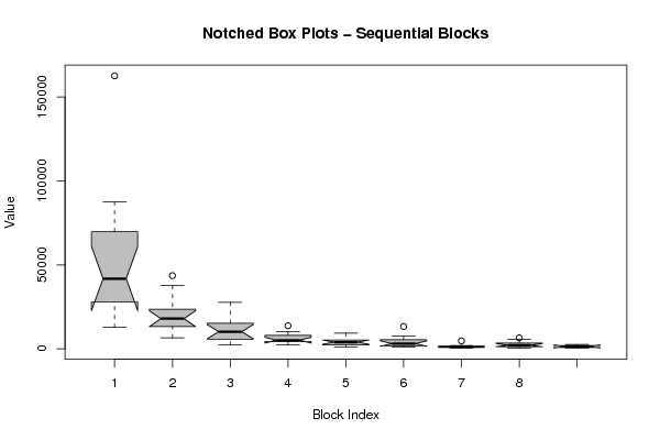
| Title produced by software | Mean Plot | ||||||||||||||||||||
| Date of computation | Tue, 30 Nov 2010 23:02:55 +0000 | ||||||||||||||||||||
| Cite this page as follows | Statistical Computations at FreeStatistics.org, Office for Research Development and Education, URL https://freestatistics.org/blog/index.php?v=date/2010/Dec/01/t1291158358eyfigdy5gycl52i.htm/, Retrieved Sun, 05 May 2024 14:23:31 +0000 | ||||||||||||||||||||
| Statistical Computations at FreeStatistics.org, Office for Research Development and Education, URL https://freestatistics.org/blog/index.php?pk=103873, Retrieved Sun, 05 May 2024 14:23:31 +0000 | |||||||||||||||||||||
| QR Codes: | |||||||||||||||||||||
|
| |||||||||||||||||||||
| Original text written by user: | |||||||||||||||||||||
| IsPrivate? | No (this computation is public) | ||||||||||||||||||||
| User-defined keywords | |||||||||||||||||||||
| Estimated Impact | 163 | ||||||||||||||||||||
Tree of Dependent Computations | |||||||||||||||||||||
| Family? (F = Feedback message, R = changed R code, M = changed R Module, P = changed Parameters, D = changed Data) | |||||||||||||||||||||
| - [Mean Plot] [] [2010-11-25 21:20:50] [1c63f3c303537b65dfa698074d619a3e] - PD [Mean Plot] [Paper - Notched b...] [2010-11-30 23:02:55] [ffc0b3af89e3f152a248771909785efd] [Current] | |||||||||||||||||||||
| Feedback Forum | |||||||||||||||||||||
Post a new message | |||||||||||||||||||||
Dataset | |||||||||||||||||||||
| Dataseries X: | |||||||||||||||||||||
162556 29790 87550 84738 54660 42634 40949 45187 37704 16275 25830 12679 18014 43556 24811 6575 7123 21950 37597 17821 12988 22330 13326 16189 7146 15824 27664 11920 8568 14416 3369 11819 6984 4519 2220 18562 10327 5336 2365 4069 8636 13718 4525 6869 4628 3689 4891 7489 4901 2284 3160 4150 7285 1134 4658 2384 3748 5371 1285 9327 5565 1528 3122 7561 2675 13253 880 2053 1424 4036 3045 5119 1431 554 1975 1765 1012 810 1280 666 1380 4677 876 814 514 5692 3642 540 2099 567 2001 2949 2253 6533 1889 3055 272 1414 2564 1383 | |||||||||||||||||||||
Tables (Output of Computation) | |||||||||||||||||||||
| |||||||||||||||||||||
Figures (Output of Computation) | |||||||||||||||||||||
Input Parameters & R Code | |||||||||||||||||||||
| Parameters (Session): | |||||||||||||||||||||
| par1 = 0 ; | |||||||||||||||||||||
| Parameters (R input): | |||||||||||||||||||||
| par1 = 12 ; | |||||||||||||||||||||
| R code (references can be found in the software module): | |||||||||||||||||||||
par1 <- as.numeric(par1) | |||||||||||||||||||||