Free Statistics
of Irreproducible Research!
Description of Statistical Computation | |||||||||||||||||||||
|---|---|---|---|---|---|---|---|---|---|---|---|---|---|---|---|---|---|---|---|---|---|
| Author's title | |||||||||||||||||||||
| Author | *Unverified author* | ||||||||||||||||||||
| R Software Module | rwasp_sdplot.wasp | ||||||||||||||||||||
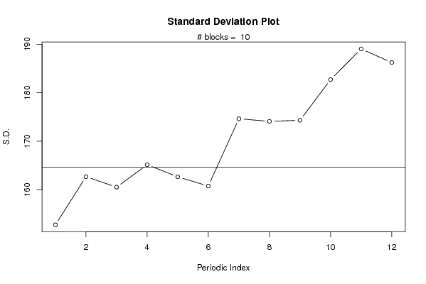
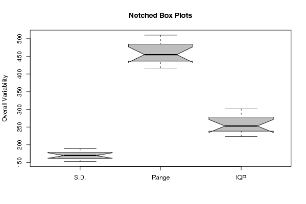
| Title produced by software | Standard Deviation Plot | ||||||||||||||||||||
| Date of computation | Mon, 16 Aug 2010 09:45:03 +0000 | ||||||||||||||||||||
| Cite this page as follows | Statistical Computations at FreeStatistics.org, Office for Research Development and Education, URL https://freestatistics.org/blog/index.php?v=date/2010/Aug/16/t1281951912p4g5f8jkpz5at18.htm/, Retrieved Thu, 16 May 2024 23:50:36 +0000 | ||||||||||||||||||||
| Statistical Computations at FreeStatistics.org, Office for Research Development and Education, URL https://freestatistics.org/blog/index.php?pk=78947, Retrieved Thu, 16 May 2024 23:50:36 +0000 | |||||||||||||||||||||
| QR Codes: | |||||||||||||||||||||
|
| |||||||||||||||||||||
| Original text written by user: | |||||||||||||||||||||
| IsPrivate? | No (this computation is public) | ||||||||||||||||||||
| User-defined keywords | |||||||||||||||||||||
| Estimated Impact | 134 | ||||||||||||||||||||
Tree of Dependent Computations | |||||||||||||||||||||
| Family? (F = Feedback message, R = changed R code, M = changed R Module, P = changed Parameters, D = changed Data) | |||||||||||||||||||||
| - [Histogram] [Bezoekers per maand] [2010-08-16 07:07:56] [3d41945eca20332ad7c135bac91a27a3] - RMP [Standard Deviation Plot] [aa] [2010-08-16 09:45:03] [5e78ed906b09bab42b8ec3dd93b6358a] [Current] | |||||||||||||||||||||
| Feedback Forum | |||||||||||||||||||||
Post a new message | |||||||||||||||||||||
Dataset | |||||||||||||||||||||
| Dataseries X: | |||||||||||||||||||||
556 555 554 552 572 571 556 546 547 547 548 550 555 549 555 550 566 573 543 535 542 541 535 536 548 546 548 548 561 563 527 527 541 534 522 527 539 533 532 519 538 542 503 502 522 511 492 500 509 511 505 493 518 518 474 471 483 461 439 446 461 449 441 424 447 448 404 403 411 386 359 370 385 369 368 352 378 383 334 323 330 303 275 284 301 281 284 272 297 300 240 236 247 218 192 201 223 197 195 175 197 204 142 142 151 127 100 114 139 112 123 108 132 140 76 71 81 57 38 46 | |||||||||||||||||||||
Tables (Output of Computation) | |||||||||||||||||||||
| |||||||||||||||||||||
Figures (Output of Computation) | |||||||||||||||||||||
Input Parameters & R Code | |||||||||||||||||||||
| Parameters (Session): | |||||||||||||||||||||
| Parameters (R input): | |||||||||||||||||||||
| par1 = 12 ; | |||||||||||||||||||||
| R code (references can be found in the software module): | |||||||||||||||||||||
par1 <- as.numeric(par1) | |||||||||||||||||||||