Free Statistics
of Irreproducible Research!
Description of Statistical Computation | |||||||||||||||||||||||||||||||||||||||
|---|---|---|---|---|---|---|---|---|---|---|---|---|---|---|---|---|---|---|---|---|---|---|---|---|---|---|---|---|---|---|---|---|---|---|---|---|---|---|---|
| Author's title | |||||||||||||||||||||||||||||||||||||||
| Author | *Unverified author* | ||||||||||||||||||||||||||||||||||||||
| R Software Module | rwasp_fitdistrcauchy.wasp | ||||||||||||||||||||||||||||||||||||||
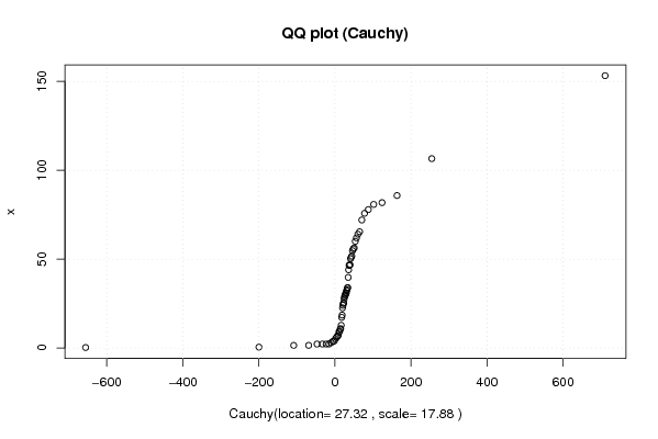
| Title produced by software | Maximum-likelihood Fitting - Cauchy Distribution | ||||||||||||||||||||||||||||||||||||||
| Date of computation | Fri, 16 Apr 2010 12:28:29 +0000 | ||||||||||||||||||||||||||||||||||||||
| Cite this page as follows | Statistical Computations at FreeStatistics.org, Office for Research Development and Education, URL https://freestatistics.org/blog/index.php?v=date/2010/Apr/16/t1271420942r3ijrc7lz8kz13n.htm/, Retrieved Thu, 25 Apr 2024 19:15:04 +0000 | ||||||||||||||||||||||||||||||||||||||
| Statistical Computations at FreeStatistics.org, Office for Research Development and Education, URL https://freestatistics.org/blog/index.php?pk=74651, Retrieved Thu, 25 Apr 2024 19:15:04 +0000 | |||||||||||||||||||||||||||||||||||||||
| QR Codes: | |||||||||||||||||||||||||||||||||||||||
|
| |||||||||||||||||||||||||||||||||||||||
| Original text written by user: | |||||||||||||||||||||||||||||||||||||||
| IsPrivate? | No (this computation is public) | ||||||||||||||||||||||||||||||||||||||
| User-defined keywords | B611,steven,coomans,cauchy,thesis | ||||||||||||||||||||||||||||||||||||||
| Estimated Impact | 219 | ||||||||||||||||||||||||||||||||||||||
Tree of Dependent Computations | |||||||||||||||||||||||||||||||||||||||
| Family? (F = Feedback message, R = changed R code, M = changed R Module, P = changed Parameters, D = changed Data) | |||||||||||||||||||||||||||||||||||||||
| - [Maximum-likelihood Fitting - Cauchy Distribution] [B611,steven,cooma...] [2010-04-16 12:28:29] [d41d8cd98f00b204e9800998ecf8427e] [Current] | |||||||||||||||||||||||||||||||||||||||
| Feedback Forum | |||||||||||||||||||||||||||||||||||||||
Post a new message | |||||||||||||||||||||||||||||||||||||||
Dataset | |||||||||||||||||||||||||||||||||||||||
| Dataseries X: | |||||||||||||||||||||||||||||||||||||||
46.426 46.855 153.135 64 31 2.25 2.25 2.3 22.6 1.5 10.65 34 81.75 106.5 0.525 24.025 5.25 9 12.8 25.05 0.3 75.75 54.75 1.526 30.993 3.752 17.25 9.2 50.25 2.25 3.95 60 55.8 6.75 61.95 7.025 85.75 18.525 6 25.35 46.775 51.025 30 3 30 44 80.75 27.5 39.725 29.25 32.725 56.25 28.65 51.75 32.26 72 65.4 33.75 77.85 10.875 | |||||||||||||||||||||||||||||||||||||||
Tables (Output of Computation) | |||||||||||||||||||||||||||||||||||||||
| |||||||||||||||||||||||||||||||||||||||
Figures (Output of Computation) | |||||||||||||||||||||||||||||||||||||||
Input Parameters & R Code | |||||||||||||||||||||||||||||||||||||||
| Parameters (Session): | |||||||||||||||||||||||||||||||||||||||
| Parameters (R input): | |||||||||||||||||||||||||||||||||||||||
| R code (references can be found in the software module): | |||||||||||||||||||||||||||||||||||||||
library(MASS) | |||||||||||||||||||||||||||||||||||||||